Showing posts with label PIC. Show all posts

Wednesday, August 28, 2024

Neon bar-graph VSWR/Power meter using the ИН-13 (a.k.a "IN-13") "Nixie" - Part 1 (of 3)

Figure 1:
Power/VSWR meter using
ИН-13 (a.k.a. "IN-13") neon bar-graph indicators.
Click on the image for a larger version.
(Be sure to read Part 2 of this article - LINK).
 
Several years ago I bought some Soviet-era neon bar-graph displays - mainly because I thought that they looked cool, but I didn't have any ideas for a specific project.  
 
After mulling over possible uses for these things for a year or so - trying to think of something other than the usual audio VU meter or thermometer - I decided to construct a visual watt/VSWR indicator for amateur radio HF use.
 
* * *
 
I actually bought two different types of these bar-graph tubes:
  • The ИН-9 (a.k.a. "IN-9").  This tube is 5.5" (140mm) long and 0.39" (10mm) diameter.  It has two leads and the segments light up sequentially - starting from the end with the wires - as the current increases.
  • The ИН-13 (a.k.a "IN-13").  This neon bar-graph tube is about 6.3" (160mm) long and 0.39" (10mm) diameter.  Like the ИН-9 its segments light up sequentially with increasing current but it has a third lead - the "auxiliary cathode" - that is tied to the negative supply lead via a 220k resistor that provides a "sustain" current to make it work more reliably at lower currents.
Note:  It would be improper to refer to these as "Nixies" as that term refers to a specific type of numeric display - which these are not.  Despite this, the term is often applied - likely for "marketing" purposes to get more hits on search engines.

Figure 2:
A pair of ИН-13 neon indicator tubes.  These tubes are
slightly longer than than the
ИН-9 tubes and have three leads
Click on the image for a larger version.
For a device that is intended to indicate specific measurements, it's important that it is consistent, and for these neon indicators, that means that we want the bar graph to "deflect" the same amount anytime the same amount of current is applied to it.  In perusing the specifications of both the 
ИН-9 and  ИН-13 it appeared that the  ИН-13 would be more suitable for our purposes.

This project would require two tubes:
  • Forward power indicator.  This would always indicate the forward RF power as that was that's something that is useful to know at any time during transmitting.
  • Reverse power/VSWR.  This second tube would switchable between reverse power, using the same scale as the forward power display, and VSWR - a measurement of the ratio between forward and reverse power and a useful indicator of the state of the match to the antenna/feedline.
Driving the tubes
  
"Because physics", gas discharge tubes require quite a bit of voltage to "strike" (e.g. light up) and these particular tubes need for their operation about 140 volts - a "modestly high" voltage at low current - only a few milliamps (less than 5) per tube, peak.

Figure 3:
Test circuit to determine the suitability of various inductors and transistors
and to determine reasonable drive frequencies.  Diode "D" is a high-speed,
high-voltage diode, "R" can be two 10k 1 watt resistors in parallel and
"Q" is a power FET with suitably high voltage ratings (>=200 Volts)
and a gate turn-on threshold in the 2-3 volt range so that it is suitable
to be driven by 5 volt logic.  V+ is from a DC power supply that is
variable from at least 5 volts to 10 volts.  The square wave drive, from a
function generator, was set to output a 0-5 volt waveform to
make certain that the chosen FET could be properly driven by a 5 volt
logic-level signal from the PIC as evidenced by it not getting perceptibly
warm during operation.
Generating high voltage from a low is one of the aspects that I tackled in a previous project on this blog when I built a high voltage power supply for the Zenith Transoceanic:  You can read about that here - A microcontroller-based A/B Battery replacement for the Zenith TransOceanic H-500 radio, with filament regulation - link.
 
The method used for this project and the aforementioned Zenith radio is  boost-type converter as depicted in Figure 3.  The switching frequency must be pretty high -  typically in the 5-30 kHz range if one wishes to keep the inductance and physical size of that inductor reasonably small.

As in the case of the Zenith Transoceanic project, I used the PWM output of the microcontroller - a PIC - to drive the voltage converter with a frequency in the range of 20-50 kHz.  For our needs - generating about 140 volts at, say, 15 milliamps maximum, I knew (from experience) that a 220uH choke would be appropriate.  Figure 4, below, shows the as-built boost circuit.
Figure 4:
The voltage boost converter section showing the transistor/inductor, rectification/filtering and
voltage divider circuitry.

Description:
 
Q301 is a high-voltage (>=200 volt) N-channel MOSFET - this one being pulled from a junked PC power supply (the particular device isn't critical) which is driven by a square wave on the "HV_PWM" line from the microcontroller:  R301, the 10k resistor, keeps the transistor in the "off" state when the controller isn't actively driving it (e.g. start-up).  L301, a 220uH inductor, provides the conversion:  When Q301 is on, the bottom end is shorted to ground causing a magnetic field to build up and when Q301 is turned off, this field collapses, dumping the resulting voltage through D301, which is a "fast" high voltage diode designed for switching supplies - a 1N4000 series diode would not be a good choice in this application as it's quite "slow".
 
R304, a 33k resistor, is used to provide a minimum load of the power supply, pulling about 4.25 mA at 140 volts:  This "ballast" improves the ability of the supply to be regulated as the difference between "no load" (the neon bar-graphs energized, but with no "deflection") and full load (all segments of the tubes illuminated) is less than 4:1.  The resistive divider of R302 and R303 is used to provide a sample of the output voltage to the microcontroller, yielding about 2.93 volts when the output is at 140 volts.  The reader will, by now, likely have realized that I could have used R304 as part of the voltage divider - but since the value of this resistor was determined during testing, I didn't bother removing R302/R303 when I was done:  Anyway, resistors are cheap!
 
Setting the current:
 
Having the 140 volt supply is only the first part of the challenge:  As these tubes use current to set the "deflection" (e.g. number of segments) we need to be able to precisely set this parameter - independent of the voltage - to indicate a value with any reasonable accuracy.  For this we'll use a "current sink".
 
Figure 5:
The precision current sinks that drive the neon tubes precisely based on PWM-derived voltage.
Click on the image for a larger version.
 
Figure 5, above, shows the driving circuits for the two tubes using the "precision current sink".  Taking the top diagram as our example, we see that the inverting input of the op-amp (U401c) is connected to the junction of the emitter of Q401 and resistor R406.  As is the wont of an op amp, the output will be driven high or low as needed to try to make the voltage (from the microcontroller) at pin 10 match that of pin 9 - in this case, based on feedback from the sense resistor, R406.

What this means is that as the transistor (Q401) is turned on, current will flow from the tube, through it and into R406 meaning that the voltage across R406 is proportional to the voltage on pin 10.  It should be noted that current through R406 will include the current into the base - but this can be ignored as it will be only a tiny fraction (a few percent at most) of the total current.  It's worth noting that this circuit is insensitive to the voltage - at least as long as such current can be sunk - making it ideal for driving a device like the ИН-13 (or ИН-9) in which its intended operation is dependent on the current rather than the operating voltage.

At this point it's worth noting that the driving voltages from the microcontroller ("FWD_PWM" and "REV_PWM") are not plain DC voltages, but rather from the 10 bit PWM outputs of the microcontroller.  The use of a 10k resistor and 100nF (0.1uF) capacitors (R405 and C406, respectively) "smooth" the square-ish wave PWM into DC.
 
Q401 and Q402 were, again, random transistors that I found in scrapped power supplies, but since there's at least 70 volts drop across the tube, about any NPN transistor rated to withstand at least 80 volts should suffice.  It's also worth noting the presence of R407 and R409, which provides the "sustain" current on the "auxiliary" cathode.
Figure 6:
An exterior view of the tandem coupler module.
Visible is the top shield and the three feedthrough
capacitors used to pass voltage and block RF.
Click on the image for a larger version.

RF sensing

For sensing forward and reflected power I decided to use an external "sensing head" that was connected inline with the radio, on the "tuner" side of the feedline.  

For sensing power in both directions I chose the so-called "Tandem" coupler which consists of a through-line sampler in which a short length of coaxial cable carrying the transmit power (T1 in the diagram of Figure 7) passes through a toroidal core - using some of the original cable's braid grounded at just one end as a Faraday shield.  An identical transformer (T2) is connected across the first (T1) for symmetry.

When carefully constructed this arrangement has quite good intrinsic directivity and a wide frequency range.  Figure 6 shows the diagram of this section.

Figure 7:
Schematic diagram of the "Tadem" coupler.  A bidirectional coupler sends power to
separate AD8307 logarithmic amplifiers - one for forward and the other for reverse.
The outputs, expressed in "volts/dB" are sent to the microcontroller.
Click on the image for a larger version.

The RF sensing outputs of the second tandem coupler (T2) then goes through resistive voltage dividers (R606/R607 for the reverse sample and R603/604 for the forward sample) to a pair of Analog Devices AD8307 logarithmic amplifiers - one for forward power and the other for reverse - to provide a DC voltage that is logarithmically proportional to the detected RF power.  This voltage is then coupled through series resistors (for both RF and DC protection) R605/R608 and to the outside world using feedthrough capacitors.

The use of a logarithmic amplifier precludes the need to have range switching on power meter as RF energy from well below a watt to well over 2000 watts can be represented with only a few volts swing.  Looking carefully at Figure 6 one can see a label that notes that the response of the AD8307 is about 25 millivolts per dB - and this applies across the entire power range of a few hundred milliwatts to 2000 watts.

All of this circuitry is mounted in a box constructed of circuit board material and connected to the display unit with an umbilical cable that conveys power and ground along with the voltages that indicates forward and reflected power.

Figure 8:
An inside view of the Tandem Match (sense unit) showing
the coupling lines, internal shielding and AD8307 boards.
Click on the image for a larger version.
Figure 8 shows the as-built "sense unit" and the two coaxial sense lines are clearly visible.  As can be seen, the "main line" coupler is physically separated and shielded from the secondary sense line, using PTFE ("Teflon") feedthrough lines to pass the signals.

The AD8307 detectors themselves can be seen at the left and right edges of the lower half of the unit, built on small pieces of perfboard.  All signals - including the 12 volt power and the DC voltages of the output pass through 4000pF feedthrough capacitors to prevent both ingress and egress of RF energy which could find its way into the '8307 detectors and skew readings.

* * * * *

In a future posting (Part 2) we'll talk about the final design and integration of this project.


This page stolen from ka7oei.blogspot.com

[END]


Tuesday, September 27, 2022

Using an ATX computer power supply to run KiwiSDRs - and as a general purpose 5 and 12 volt supply

At the Northern Utah WebSDR (link) we run a number of KiwiSDR receivers.  These receivers, which are inherently broadband (10 kHz to 30 MHz) allow a limited number of users to tune across the bands, allowing reception on frequencies that are not covered by the WebSDR servers.

At present there are six of these receivers on site:  Three are connected to the TCI-530 Omnidirectional antenna (covering 630-10 meters - 2200 meters is included via a separate E-field whip), two are on the east-pointing log-periodic beam antenna (which overs 40-10 meters) and the newest is connected to the northwest-pointing log-periodic beam antenna (which covers 30-10 meters).

Figure 1:
Power supply in a PC case!
The PC case housing the power supply was repurposed -
because, why not?
Click for larger version
The power requirements of a KiwiSDR are modest, being on the order of 600-800 mA, but the start-up current can briefly exceed 1.25 amps.  Additionally, they do not start up reliably if the voltage "ramps up" rather slowly - a problem often exacerbated by the fact that the extra current that they draw upon power-up can cause a power supply to "brown out".

Up to this point we had been running 5 KiwiSDRs:  Three of them were powered by a pair of 5 volt, 3 amp linear power supplies that are "dioded-ANDed" together to form a 6 amp power supply and the other two KiwiSDRs were powered from a heavily-filtered 5-volt, 3 amp switching power supply.

In recent months, the dual 3 amp linear supply had become problematic, not being able to handle the load of the three KiwiSDRs, so we had to power down KiwiSDR #3.  With the recent installation of the northwest-pointing log periodic antenna, we were also looking toward installing another KiwiSDR for that antenna and we were clearly out of power supply capacity.

Using an ATX supply as a general-purpose power supply - it's not just the green wire!

If you look around on the Web, you'll see suggestions that you just "ground the green wire" to turn on an ATX supply, at which point you may use it as a general-purpose supply.  While grounding the green wire does turn it on, it's not as simple as that - particularly if you leave the power supply unattended.

For example, what if there is a brief short on the output while you are connecting things, or what if the power browns out (or turns off) for just the "wrong" amount of time.  These sorts of things do happen, and can "trip out" the power supply and it may never restart on its own.

With the site being remote, we couldn't afford for this to happen - so you'll see, below, how we remedied this.

Putting together another power supply:

With six KiwiSDRs, the power supply requirements were thus:

  • 5 amps continuous, making the assumption that a KiwiSDR's average current consumption would be about 830 mA - a number with generous overhead.
  • 9 amps on start-up, presuming that each KiwiSDR would briefly consume 1.5 amps upon power-up, again a value with a bit of overhead.
  • The power supply must not exhibit a "slow" ramp-up voltage as the KiwiSDRs did not "like" that.

In looking around for a power supply on which to base the design, the obvious choice was an computer-type ATX power supply.  Fortunately, I have on-hand a large number of 240 watt ATX supplies with active power factor correction which are more than capable of supplying the current demands, being rated for up to 22 amps load on the 5 volt supply - more than enough headroom as I would be needing less than half of that, at least with the currently-planned usage.

Circuit description:

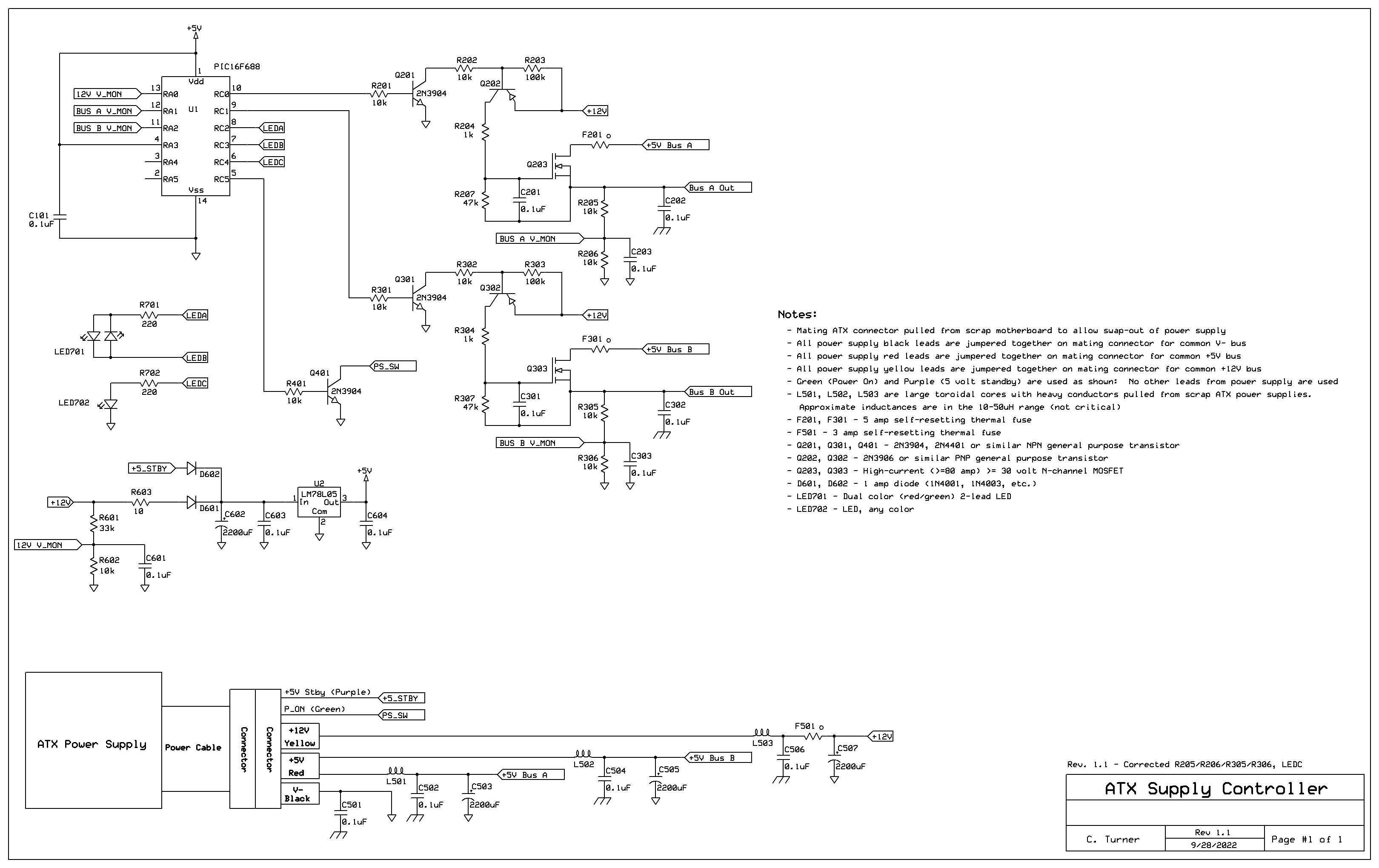
Refer to the schematic in Figure 2 for components in the description.

Added filtering:

While these power supplies were already known to be adequately RF-clean (important for a receive site!) from their wide use for the WebSDR servers because we would be conducting the DC outputs outside the box - and to receivers - I felt it important that additional filtering be added.  Having scrapped a number of PC power supplies in the past, I rummaged around in my box of random toroids and found two that had probably come from old PC power supplies, wound with heavy wire consisting of 4 or 5 strands in parallel.  These inductors measured in the area 10s of microHenries, enough for HF filtering when used with additional outboard capacitance.

These filter networks were constructed using old-fashioned phenolic terminal lug strips.  These consist of a row of lugs to which components are soldered - typically with one or two of the lugs used for mounting, and also "grounding".  Rather than mount these lugs using a drill and screw, they were soldered to the steel case itself - something easily done by first sanding a "bare" spot on the case to remove any paint or oxide and then using an acid-core flux - cleaning it up afterwards, of course!

The heavier components (inductors, capacitors) were mechanically secured using RTV (silicone) adhesive to keep them from moving around - and to prevent the possibility of the inductor's wire from touching the case and chafing.

Looking at the schematic you may note that  C202, C302, C501, C502 and C503 are connected to a "different" ground than everything else.  While - at least for this power supply - the "Common" (black) wire is internally connected to the case, it's initially assumed that this lead - which comes from the power supply - may be a bit "noisy" in terms of RF energy, so they are RF bypassed to the case of the power supply.  This may have been an unneeded precaution, but it was done nonetheless.

Connectorizing and wiring the power supply:

The ATX power connector was extracted from a defunct PC motherboard to allow the power supply itself to be replaced in the future if needed.  On this connector, all of the pins corresponding with the 5 volt (red wires), 12 volt (yellow wires) and ground (black wires) were bonded together to form three individual busses and heavy (12 AWG) wires were attached to each:  This was done to put as many of the wires emerging from the power supply in parallel with each other to minimize resistive losses. 

The green wire (the "power" switch) and purple wire (the 5 volt "standby") were brought out separately as they would be used as well - and the remainder of the pins (3.3 volt, -12 volt, -5 volt, "power good", etc.) were flooded with "hot melt" glue to prevent anything from touching anything else that it shouldn't.

The 5 volt supply was split two ways - each going to its own L/C filter network (L501, L502, C502, C503, C504, C505) as shown in the schematic, this being done to reduce the total current through the inductor - both to minimize resistive losses, but also to reduce the magnetic flux in each inductor, something that could reduce its effective inductance.

Although I don't have immediate plans to use the 12 volt supply, a similar filter (L503, C506, C507) was constructed for the 12 volt supply lead.  On the output side of the 12 volt filter, a 3 amp self-resetting thermal fuse (F501) was installed to help limit the current should a fault occur. 

About the self-resetting fuses:

 These fuses - which physically look like capacitors - operate by having a very low resistance when "cold".  When excess current flows, they start to get warm - and if too much current flows, they get quite hot (somewhere above 200F, 100C) and their internal resistance skyrockets, dropping the current to a fraction of its original value:  It's this current flow and their heat that keeps the resistance high.

It's worth noting that these fuses don't "disconnect" the load - they just reduce the current considerably to protect whatever it is connected to it.  Since, when "blown", they are hot, they must be mounted "in the clear" away from nearby objects that could be damaged by the heat - and also to prevent lowering of their trip current by trapping heat or being warmed by another component - such as another such fuse.  

It should be noted that if the outputs - either 5 or 12 volts - are "hard shorted", the thermal fuse may not react quickly enough prevent the power supply from detecting an overcurrent condition and shutting down.  As an output short is not expected to be a "normal" occurrence, this behavior is acceptable - but it will require that the power supply be restarted to recover from shutdown, as described below.

In the case of the KiwiSDRs, they are connected with fairly long leads (about 6 feet, 2 meters) and often have enough internal resistance to reduce the current below the power supply's overcurrent limit and rather than allowing the full current of the power supply (which could be more than 20 amps) to flow through and burn up this cable, the fuse will trip as it should, protecting the circuit.  To "reset" the fuse, the current must be removed completely for long enough for the device to cool - something that is done with the 5 volt supplies as we'll see, below.

The controller:

As mentioned earlier, if you look on the web, you'll see other power supply projects that use an ATX power supply as a benchtop power source and most of those suggest that one simply connect the green (power on) wire to ground to turn it on - but this isn't the whole story.  In testing the power supply, I noticed two conditions in which doing this wouldn't be enough:

  • Shorting a power supply output.  If the output of a good-quality ATX power supply is shorted, it will immediately shut down - and stay that way until the mains power is removed (for a minute or so) or the power supply is "shut off" by un-grounding the green wire for a few seconds before reconnecting to "restart" the power supply.
  • Erratic mains power interruption.  It was also observed that if the mains power was removed for just the right amount of time, the power supply would also shut down and would not restart on its own.  It took the same efforts as recovering from an output short to restart the power supply.

Since this power supply would be at the WebSDR site - an unmanned location in rural, northern Utah - it would require additional circuitry to make this power supply usable.

Fortunately, an ATX power supply has a second built-in power supply that is independent of the main one - the "standby" power supply.  This is a low-power 5 volt supply that is unaffected by what happens to the main supply (e.g. not controlled by the power switch and not affected if it "trips off") and can be used to power a simple microcontroller-based board that can monitor and sequence the start-up of the main power supply.  For this task I chose the PIC16F688, a 14 pin microcontroller with A/D conversion capability and a built-in clock oscillator.

As seen in the schematic, the "5 volt standby" is dioded-ORed (D601, D602) with the main power supply (12 volts) so that it always gets power - from either the 5 volt standby, or from the 12 volt output - when mains is applied.  R603 and capacitor C602 provide a degree of protection to the voltage regulator should some sort of "glitch" appear on the 12 volt supply - possibly due to the 5 volt load being abruptly disconnected (or connected) as the 5 and 12 volt supplies are "co-regulated" in the sense that it's really only the 5 volt output that is being regulated well - the 12 volt power supply's output is pretty much a fixed ratio to the 5 volt and doesn't really have much in terms of separate regulation.

It should be noted that when operating from the standby +5 volt power source, the voltage from U2 (the 5 volt regulator) is on the order of 3 volts or so (drop through D602 and U2) but this is comfortably above the "brownout" threshold of the PIC, which is around 2.5 volts, so there isn't really a worry that the low-voltage brownout detector will trigger erroneously and prevent start-up.  If it had, I would have simply moved the cathode side of D602 to the +5V side of U2.

Figure 3: 
Inside the case!
Top right:  12 volt supply filtering and thermal fuse
Upper-middle:  Dual 5 volt filtering
Lower middle:  Controller board with FET switches
and thermal fusing.
The ATX power supply is in the lower-left corner.
Click on the image for a larger version.
Because the PIC microcontroller can monitor the 12 volt supply (via R601/R602) it "knows" when the main ATX supply is turned off.  Through the use of an NPN transistor (Q401) - the collector of which can be used to "ground" the green "power on" line, the controller can turn the main power supply on and off as follows:
  • When the microcontroller starts up, it makes sure that the ATX "power on" wire is turned off (e.g. un-grounded).  This is done by the microcontroller turning off Q401.
  • After a 10 second delay, it turns on the power supply by turning on Q401.

It also monitors the power supply to look for a fault.  If either the 5 or 12 volt output is shorted or faults out, both power supply outputs (but not the 5 volt "standby" output) disappear.

  • If, while running, the monitored 12 volt supply (via R601/R602 and "12V V_MON") drops below about half the voltage (e.g. trips out) the "power on" wire is turned off using Q401, disabling the ATX power supply.
  • A 10 second delay is imposed before attempting to turn the power supply back on.
  • Once the power supply is turned back on, monitoring of the voltage resumes.

In practice, if there is a "hard" short on the output, the power supply will attempt to restart every 10 seconds or so, but remember that a short on an output could occur with ANY sort of power supply, so this isn't a unique condition.

5 volt output sequencing and monitoring:

The other function of the controller is to sequence and monitor the 5 volt outputs.  As mentioned earlier, it was noted that the KiwiSDRs do not "like" a slow voltage ramp-up so a FET switch is employed to effect a rapid turn-on - and since there are two separately-filtered 5 volt busses, there are two such switches.  In order to reduce the peak current caused when the load is suddenly connected, each of these busses is turned on separately, a 10 second delay between the two of them.

The N-channel FET switches (Q203, Q303) are controlled by an NPN (Q201, Q301) transistor being turned on by the microcontroller which, in turns, "pulls" the base of a PNP transistor (Q202, Q302) low via a base resistor (R202/R302), turning it on - and other resistors (R203, R303) assure that these transistors are turned off as needed.

With the emitter of the PNP connected to the 12 volt supply, the gate voltage of the FET is approximately 7 volts higher than the drain voltage, assuring that it is turned on with adequately low resistance.  Capacitors (C201, C301) are connected between the FET's gates and sources to suppress any ringing that might occur when the power is turned on/off and as a degree of protection against source-gate voltage spikes while the 47k resistor (R207/R307) assure that the FET gets turned off.

The use of P-channel FETs was considered, but unless special "logic level" threshold devices were used, having only 5 volts between the gate and drain wouldn't have turned them fully "on" unless the -5 or -12 volt supply from the power supply was also used.  While this would certainly have been practical, N-channel FETs are more commonly available.

Figure 2: 
Schematic of the ATX controller with power supply filtering, voltage monitoring, and control.
See the text for a description.
Click on the image for a larger version.

In series with the 5 volt supply and the FET's source is a 5 amp self-resetting thermal fuse to limit current.  Should an overload (more than 5-ish amps) occur on the output bus, this fuse will heat up and go to high resistance, causing the output voltage to drop.  If this occurs, the microcontroller, which is using its A/D converter to look at the voltage divider on the outputs (R205/R206 for the "A" channel, R305/R306 for the "B" channel) will detect this dip in voltage and immediately turn off the associated FET.  After a wait of at least 10 seconds - for the fault to be cleared (in the event that it is momentary) and to allow the thermal fuse to cool off and reset - the power will be reconnected.  If there continues to be a fault, the reset time is lengthened (up to about 100 seconds) between restart attempts.

Finally, the status of the power supply is indicated by a 2-lead dual-color (red/green) LED (LED701) mounted to be visible from the front panel.  During power supply start-up, it flashes red, during the time delay to turn on the power supplies it is yellow, when operation is normal it is green - and if there is a fault, it is red.  Optionally, another LED (LED702) can be mounted to be visible:  This LED is driven with the algorithm that causes it to "breath" (fade on and off - and on, and off...) to indicate that "something" was working.  I simply ran out of time, so I didn't install it.

* * *

This power supply was put together fairly quickly, so I didn't take as many pictures as I usually would - and I omitted taking pictures of the back panel where the power supply connections are made.  Perhaps it's just as well as while I used a good-quality screw-type barrier strip, it was mounted to a small piece of 1/4" (6mm) thick plywood that was epoxied into the rectangular hole where one would connect peripherals to the motherboard.

As you would expect, the terminals are color-coded (using "Sharpies" on the wood!) and appropriately labeled.  While not pretty, it's functional!

(Comment:  The photo in Figure 3 was taken before I added the circuit to control the "Power On" wire (e.g. Q401) and the diode-OR power (D601, D602) - and it shows the dual-color LED on the board during testing.)

If you are interested in the PIC's code, drop me a note.

This page stolen from ka7oei.blogspot.com

[END]


Tuesday, August 30, 2022

Making a "Word Metronome" for pacing of speech

Figure 1:
The completed "Word Metronome".  There are two recessed
buttons on the front and the lights on on the left side.
Click on the image for a larger version.
One of the things that my younger brother's job entails is to provide teaching materials - and this often includes some narration.  To assure consistency - and to fall within the required timeline - such presentations must be carefully designed in terms of timing to assure that everything that should be said is within the time window of the presentation itself.

Thus, he asked me to make a "word metronome" - a stand-alone device that would provide a visual cue for speaking cadence.  The idea wasn't to make the speech robotic and staccato in its nature, but rather providing a mental cue to provide pacing - something that is always a concern when trying to make a given amount of material fit in a specific time window:  You don't want to go too fast - and you certainly don't want to be too slow and run over the desired time and, of course, you don't want to randomly change your rate of speech over time - unless there's a dramatic or context-sensitive reason to do so.

To be sure, there are likely phone apps to do this, but I tend to think of a phone as a general-purpose device, not super-well suited for most of the things done with it, so a purpose-built, simple-to-operate device with visual indicators on its side that could just sit on a shelf or desk (rather than a phone, which would have to be propped up) couldn't be beat in terms of ease-of-use.

Circuitry:

The schematic of the Word Metronome is depicted in Figure 2, below:

Figure 2:
Schematic of the "Word Metronome"
(As noted in the text, the LiIon "cell protection" board is not included in the drawing).
Click on the image for a larger version.

This device was built around the PIC16F688, a 14 pin device with a built-in oscillator.  This oscillator isn't super-accurate - probably within +/-3% or so - but it's plenty good for this application.

One of the complications of this circuit is that of the LEDs:  Of the five LEDs, three of them are of the silicon nitride "blue-green" type (which includes "white" LEDs) and the other two are high-brightness red and yellow - and this mix of LED types poses a problem:  How does one maintain consistent brightness over varying voltage.

As seen in Figure 3, below, this unit is powered by a single lithium-ion cell, which can have a voltage ranging from 4.2 volts while on the charger to less than 3 volts when it is (mostly) discharged.  What this means is that the range of voltage - at least for the silicon nitride types of LEDs - can range from "more than enough to light it" to "being so dim that you may need to strike a match to see if it's on".  For the red and yellow LEDs, which need only a bit above two volts, this isn't quite the issue, but if one used a simple dropping resistor, the LED brightness would change dramatically over the range of voltages available from the battery during its discharge curve.

As one of the goals of this device was to have the LEDs be both of consistent brightness - and to be dimmable -  a different approach was required - and this required several bits of circuity and a bit of attention to detail in the programming.

The Charge Pump:

Perhaps the most obvious feature of this circuit is the "Charge Pump".  Popularized by the well-known ICL7660 and its many (many!) clones, this type of circuit may also be driven by a microcontroller and implemented using common parts.  Like its hardware equivalent, it uses a "flying capacitor" to step up the voltage - specifically, that surrounding Q1 and Q2.  In software - at a rate of several kHz - a pulse train is created, and its operation is thus:

  • Let is start by assuming that pin RC4 is set high (which turns off Q1) and pin RA4 is set low (which turns off Q2.)
  • Pin RA4 is set high, turning on Q2, which drags the negative side of capacitor C2 to ground.  This capacitor is charged to nearly the power supply voltage (minus the "diode drop") via D1 when this happens.
  • Pin RA4 is then set low and Q2 is turned off.
  • At this point nothing else is done for a brief moment, allowing both transistors to turn themselves off.  This very brief pause is necessary as pulling RC4 low the instant RA4 is set low would result in both Q1 and Q2 being on for an instant, causing "shoot through" - a condition where the power supply is momentarily shorted out when both transistors are on, resulting in a loss of efficiency.  This "pause" need only be a few hundred nanoseconds, so waiting for a few instruction cycles to go by in the processor is enough.
  • After just a brief moment pin RC4 is pulled low, turning on Q1, which then drags the negative side of C2 high.  When this happens the positive side of C2 - which already has (approximately) the power supply voltage is listed to a potential well above that of the power supply voltage.
  • This higher voltage flows through diode D3 and charges capacitor C4, which acts as a reservoir:  This voltage on the positive side of C4 is now a volt or so less than twice the battery voltage.
  • Pin RC4 is then pulled high, turning of Q1.
  • There is a brief pause, as described above to prevent "shoot through", before we set RA4 high and turn Q2 on for the next cycle.

It is by this method that we generate a voltage several volts higher than that of the battery voltage, and this gives us a bit of "headroom" in our control of the LED current - and thus the brightness.

Current limiter:

Transistors Q3 and Q4 form a very simple current limiter:  In this case it is "upside-down" from the more familiar configuration as it uses PNP transistors - something that I did for no particular reason as the NPN configuration would have been just fine.

Figure 3:
Inside the "Word Metronome".  The 18650 LiIon cell is on
the right - a cast-off from an old computer battery pack.  The
buttons on the board are in parallel with those on the case and
were used during initial construction/debugging.
Click on the image for a larger version.

This circuit works by monitoring the voltage across R3:  If this voltage exceeds the turn-on threshold of Q3 - around 0.6 volts - it will turn on, and when this does it pulls the base voltage, provided by R5, toward Q4's emitter, turning off Q3.  By this action, the current will actually come to equilibrium at that which results in about 0.6 volts across R3 - and in this case, Ohm's law tells us that 0.6 volts across 47 ohms implies (0.6/47=0.0128 amps) around 13 milliamps:  At room temperature, this current was measured to be  a bit above 14 milliamps - very close to that predicted.

With this current being limited, the voltage of the power supply has very little effect on the current - in this case, that through the LEDs which means that it didn't matter whether the LED was of the 2 or 3 volt type, or the state-of-of charge of the battery:  The most that could ever flow through an LED no matter what was 14 milliamps.

With the current fixed in this manner, brightness could be adjusted using PWM (Pulse Width Modulation) techniques.  In this method, the duty cycle ("On" time) of the LED is varied to adjust the brightness.  If the duty cycle is 100% (on all of the time) the LED will be at maximum brightness, but if the duty cycle is 50% (on half of the time) the LED will be at half-brightness - and so-on.  Because the current is held constant, no matter what by the current limiter circuit, we know that the only think that affects brightness of the LED is the duty cycle.

LED multiplexing:

The final aspect of the LED drive circuitry is the fact that the LEDs are all connected in parallel, with transistors Q5-Q9 being used to turn them on.  When wiring LEDs in parallel, one must make absolutely sure that each LED is of the exact-same type or else that with the lowest voltage will consume the most current.

In this case, we definitely do NOT have same-type of LEDs (they are ALL different from each other) which means that if we were to turn on two LEDs at once, it's likely that only one of them would illuminate:  That would certainly be the case if, say, the red and blue LEDs would turn on:  With the red's forward voltage being in the 2.5 volt area, the voltage would be too low for the green, blue or white to even light up.

What this means is that only ONE LED must be turned on at any given instant - but this is fine, considering how the LEDs are used.  The red, yellow or green are intended to be on constantly to indicate the current beat rate (100, 130 or 160 BPM, respectively) with the blue LED being flashed to the beat (and the white LED flashing once-per-minute) - but by blanking the "rate" LED (red, yellow or green) LED when we want to flash the blue or white one, we avoid the problem altogether.

Battery charging:

Not shown in the schematic is the USB battery charging circuit.  Implementing this was very easy:  I just bought some LiIon charger boards from Amazon.  These small circuit boards came with a small USB connector (visible in the video, below) and a chip that controlled both charging and "cell protection" - that is, they would disconnect the cell if the battery voltage got too low (below 2.5-2.7 volts) to protect it.  Since its use is so straightforward - and covered by others - I'm only mentioning it in passing.

Software:

Because of its familiarity to me, I wrote the code for this device in C using the "PICC" compiler by CCS Computer Systems.  As it is my practice, this code was written for the "bare metal" meaning that it interfaces directly with the PIC's built-in peripherals and porting it to other platforms would require a bit of work.

The unit is controlled via two pushbuttons, using the PIC's own pull-up resistors.  One button primarily controls the rate while the other sets the brightness level between several steps, and pressing and holding the rate button will turn it off and on.  When "off", the processor isn't really off, but rather the internal clock is switched to 31 kHz and the charge pump and LED drivers are turned off, reducing the operating current of the processor to a few microamps at most.

Built into the software, there is a timer that, if there is no button press within 90 minutes or so, will cause the unit to automatically power down.  This "auto power off" feature is important as this device makes no noise and it would be very easy to accidentally leave it running.

Below is a short (wordless!) video showing the operation of the "Word Metronome" - enjoy!


This page stolen from ka7oei.blogspot.com

[END]


Monday, January 7, 2019

Electrically driving a mechanical speedometer from a remote wheel sensor using a motor and PID loop

A friend of mine [Dan] is building a side-by-side 4 wheeler more or less from scratch using a motorcycle engine and transmission, an instrument cluster from a motorcycle, a home-built transfer case, electronic-assist steering rack from a Honda civic and a lot of custom welded aluminum.  As you might expect, this is a long-term project and has been in the works for several years, now.

Some time ago I helped him reverse-engineer all of the wires that connect to the instrument cluster and how they are to be connected to everything else, but one thing continued to vex him:  How to make the existing speedometer read correctly.
Figure 1:
The side-by-side as it was about a year ago.  It is much farther along, now.
Click on the image for a larger version.

While it may have been possible to do so with the original-type hardware, he chose not to use the existing mechanical (spinning cable) coupling of the speedometer to the drive train - and that didn't even take into account the need of providing a precise gear ratio to make everything read correctly.  Being the sort of person that I am, I suggested that I could make this happen electronically with a bit of microcontroller magic:  I'd just need pulses from the drive train.

To that end, he added eight steel screws to an aluminum disk that was on the drive shaft output to magnetically couple the sensor meaning that I would get eight pulses per revolution of the drive shaft.  Mathematically, this meant that with the 25 inch (635mm) diameter wheel and the 3.75 differential ratio that one would get approximately 6.72 pules per second per mile per hour of vehicle speed - good enough to measure even fairly slow speeds.

The trick was to be able to drive the cable input of the mechanical speedometer with some sort of motor.  While the first guess might be to use a stepper motor for this, that guess would be wrong:  At a speed of 80 miles per hour (on the high side of the speed range at which this would ever be driven!) it was determined that a motor rotation of more than 3000 RPM would be required, a bit on the fast side for a typical stepper motor - and even though it is likely that one could make it work, there was an alternative:  Employ a DC motor with a built-in tachometer winding.

As is the case with many things, EvilBay had the answer:  A Barber-Colman FYQM 63160-25-3 brush-type DC motor was procured.  After it arrived, this motor was analyzed and it was determined that the application of 12 volts produced a speedometer reading exceeding 120 miles-per-hour and also that one rotation of the shaft produced approximately 7.85 pulses (e.g. 60RPM = 7.85Hz).  I have no idea how that fractional number of pulses per rotation occurs unless there is some internal gearing for the tachometer, but I can't detect any evidence of "gear meshing".

Dan was able to attach the motor to the speedometer with an adapter that he'd machined so I went to work on constructing a circuit that would drive it - see below.

Figure 2:
Schematic diagram of the described circuit.
Click on the image for a larger version.
Circuit description:

Pulse amplifier/detector

The operation of the circuit itself is fairly straightforward.  Starting with the pick-up coil inputs, let's look at the "Motor Tach In" circuit:  The other circuit for detecting the pulses from the wheel sensor is identical and operates in the same way.

The motor has an internal pick-up coil that outputs an AC signal that, to some extent, has an amplitude that is proportional to its rotational speed, but we are interested only in the frequency of this signal.  This coil (and the one on the wheel sensor) are "floating" (e.g. no ground/chassis) reference which is helpful to minimize the pick-up of electrical noise.  Via R101/R102, the input signal passes to a pair of back-to-back diodes (D101/D102) that limit the amplitude of this signal to about 1.2 volts peak-to-peak, and this signal is then filtered/smoothed a bit with capacitor C101.

R103-R106 and U1d form a "difference" amplifier - that is, its output is proportional to the voltage difference between the two wires from the pick-up coil and somewhat less sensitive to common-mode noise on the leads.  Having a fixed gain of about 5, this stage also amplifies the signal, yielding about 6 volts peak-to-peak maximum.  At very low speeds (several dozen RPM) the output voltage of the pick-up coil is very low - only a few 10s of millivolts - so this amplification is necessary.

The next stage (R107, U1a, R108) forms a Schmidt Trigger.  This is a short of amplifier with very high gain, but it has a built-in hysteresis meaning that there a sort of "deadband" at the center-crossing voltage:  Once the output goes "high", it takes a lower voltage to make it go "low" again than was the threshold to make it go high.  This circuit prevents "bounce" and oscillation about its threshold and once set "high" or "low" it is stuck there until the input signal crosses the threshold.

The result of this that when the motor is turning, a square wave appears on the output of U1a at the same frequency as the AC signal coming from the pick-up coil - but the amplitude at this point is constant, regardless of the speed.  The output of the Schmidt trigger circuit is then applied to Q101 via several resistors.  This simple circuit is used to act not only as a level shifter, converting the higher-voltage signal to a 5 volt signal for U2a, but it also "speeds up" the on/off transitions for the circuit that follows.

The signal from Q101 is applied to U2a which is an XOR gate wired as an inverter and buffer which is then applied to XOR gate U2b.  As can be seen, one of the inputs of U2b is tied directly to the output of U2a, but the other one passes through a resistor (R111) which has, on its other end, connected a capacitor to ground (C102) which takes a finite time to charge compared to the other input.  The result of this is that at the instant that the output of U2a changes state, the input with the resistor/capacitor combination will lag slightly, causing the output of U2b to go high for a short period before it goes low again as the capacitor is charged.  When this circuit was first constructed Q101 was omitted, but the relatively slow slew rate from the output of the op amp didn't permit the U2b pulse generator circuit to work properly - even when it had been buffered by U2a - the result being that each logic transition had multiple pulses, each being counted by the microcontroller and thus skewing the results.

The result of this is that there are two pulses for each cycle (one on the rising edge from U1a and another on its falling edge) that is input from that motor sense tachometer winding, effectively doubling the pulse rate:  Because the microcontroller's counter input is sensitive to only the rising edge of the applied signal, it will now count twice as many pulses as it normally would.  At very low speeds this increased "temporal" resolution as there will now be more pulses to count over the measurement period to determine the rotation speed.  This output pulse is very narrow - only about 2 microseconds - but the microcontroller has no problem "seeing" it with its edge-triggered input.

Microcontroller

The heart of this circuit is U3, a PIC16F1847 microcontroller.  This device was chosen because it has a wide variety of support hardware - including several externally-clockable timers and a built-in PWM (Pulse-Width Modulator) generator.  It also has a built in system clock, eliminating the need for an external crystal as well as a hardware UART so that speed information can be sent from this device on a serial data line in case we want to supply this to another device.  For speed conversion, the absolute clock rate of the processor is irrelevant because we are doing a ratiometric conversion, but any differences in the CPU clock do effect the reading of the absolute speed that might be produced - but a couple of percent variation is perfectly acceptable.


The pulses from the motor that drives the speedometer are applied to the "RB5" pin which is configured to be the input of the PIC's 16 bit hardware counter, "Timer 1" and every time a pulse occurs, this internal counter increments by one.  Another hardware timer built into the PIC is configured as an interrupt which looks at the contents of this counter 7.63 times each second and it is by looking at the difference between the count values of successive interrupts that the rotation rate can be directly measured.
Figure 3:
The completed (and working) PID controller board.  The motor's
tachometer is connected via the yellow wires (bottom-right) with
the wheel speed sensor's input (from a sensor that "sees" 8 steel bolts
coupled to the drive shaft)  being applied to the two connects
just to the left.  The red and blue wires (top left) go to the
motor's windings.
Click on the image for a larger version.

The input from the wheel sensor is very similar:  Its output pulses are applied to the "RA4" pin which is configured to be the input to the PIC's 8 bit hardware counter, "Timer 0", which also increments on each applied pulse.  Using the same 7.63 Hz interrupt the counts from this timer are used to measure the rotation rate of the the wheel via the sensor that looks at the drive shaft.

Pin "RA3" is configured to use the microcontroller's internal PWM generator.  When this pin goes high, transistor Q401 is turned on, applying power to the motor that drives the speedometer and by varying the pulse width of this signal, more or less power can be applied to the motor.  Surrounding Q401 and the motor is a network of resistors, capacitors and a diode:  These components suppress "spiky" components of the back-EMF of the motor to reduce electrical and radio-frequency noise as well as protect the components from potentially high-voltage transients that may result from the PWM switching.

Because we know the rotation rate of the motor via its tachometer coil, we can, via software, set the speed of the motor precisely - and because we also have the input from the wheel sensor (via the drive shaft) we can also know how fast the vehicle is moving.  By applying some correction factors in software, we can convert the wheel rotation rate to the motor rotation rate that will give us a correct reading on the speedometer.

Transistor Q501 and its associated resistors comprise an inverter/driver to produce a "pseudo RS-232" signal that carries serial information such as the calculated speed:  This could be used for debugging, or it may be used by some yet-to-be-built module that would use this information.

Finally, components D601, R601 and C601 form a polarity protection and filter network to suppress high-voltage transients that may appear on the vehicle's power supply while C603, C603 and U4 provide a regulated 5 volt supply for both U2 and U3 as well as being a mid-supply reference for U1.

The PID controller:

Perhaps the most complicated part if this circuit is not the hardware, but the software that takes the tachometer output from the speedometer driver motor and adjusts the PWM duty cycle.  To attain a stable and accurate result, closed-loop feedback is required - but there are several things that tend to complicate this task, including:
  • The rotational speed of the motor is not directly proportional to the PWM duty cycle.   The power supply voltage, the temperature of the motor (and the viscosity of its lubrication) and the amount of mechanical loading can affect this.  For example, when the speedometer's odometer "turns over" several digits, the motor loading is increased slightly.
  • The motor itself has significant rotational intertia.  This means that it takes a finite time for the motor to speed up or (especially) slow down when the PWM duty cycle changes.  Because of this delayed response, having some sort of "direct" feedback loop where the PWM is adjusted based on the desired rotation speed and the actual rotation speed will result in "ringing" (oscillation) about the desired value.
The PID (Proportional-Integral-Derivative)  See Ref. 1 controller algorithm is designed to accommodate this problem, being somewhat "adaptive" in that if properly implemented, it can accommodate longer-term errors while being fairly quick to respond and avoiding "ringing".  As the name implies, this controller is somewhat more complicated than a simple proportional controller, but it is still quite manageable in a microcontroller.

In many cases, a PID controller is used for position control where one inputs where a particular axis is supposed to go, using some sort of position feedback, and "output" terms are applied to the motor (or whatever) to cause movement.  In this application there are both "negative" and "positive" results related to the attained position - the positive meaning an overshoot, past the desired position and negative meaning that it isn't quite there yet - and a "negative" output might mean that the drive motor should be reversed.  In this case we have no need for a "negative" output as all we can do is speed up the motor by increasing the PWM duty cycle or slow it down by lowering the PWM duty cycle and waiting for the motor to "coast" down in RPM.

A PID controller in "pseudo" code, assuming floating-point mathematics, is as follows:

// 
// PID control
//
error = desired_speed - actual_speed;
integral = integral + (error * ITIME);
derivative = (error - error_prior)/ITIME;
output = Kp*error + Ki*integral + Kd*derivative + BIAS;
error_prior = error;

In the above:
  • desired_speed - This is the rotation speed that we would like the motor to have.  (If we were moving some sort of actuator arm, this would be used to input the desired axial position.)
  • actual_speed - This is the rotation speed of the motor being driven.  "desired_speed" and "actual_speed" are in the same units.  (If we were moving some sort of arm, this would be the actual position.)
  • error - This is the difference between the actual and desired values.  This number could be positive or negative.
  • integral - This term gets larger and larger in proportion to a constant amount of error and it acts as sort of a "memory" of the amount of error that has occurred over a longer period - which is then used to make the long-term average correct.
  • derivative - This operates on the short term, taking into account the amount of error between the current reading and the previous reading.  This helps compensate for rapid changes that might occur.
  • output - This is the "output" of the loop, the result being proportional in both amplitude and sign of how much correction to apply to make the motor do what it is supposed to do.  In the case of our PWM drive, all we can do is go to zero to cause the motor to slow down, but if we were moving some sort of actuator arm, this value might go negative to make its motor go backwards.
  • BIAS - This is a "baseline" amount when the system first starts.  As an example, if the motor doesn't start turning until the PWM value gets to 5% of maximum, it may take a short while for the loop to "ramp up", but if you set BIAS to a value just below where it starts to turn (or for a typical value the represents an acceptable "starting speed") the initial start-up of system can be quicker.  This value quickly "disappears" in normal operation.
  • ITIME - This is typically referred to as the "iteration" time, but in reality it just represents "how much" response should happen at each iteration.  If the loop is called only occasionally and "output" needs to be a fairly large value for full-speed operation, "ITIME" should be fairly large.  In short, a high number causes quicker response than a lower number if everything else is kept the same as it directly affects how much/little the integral and derivative terms change on each iteration.
  • Kp - This is the magnitude of the "proportional" (the "P" in PID) term and it sets how much a given amount of error will affect the output result.  This is a constant that must be chosen.
  • Ki - This is the magnitude of the "integral" (the "P") and it affects how much the most recent error will affect the output per each iteration.  This constant must also be chosen appropriately.
  • Kd - This is the magnitude of the "derivative" (the "D") and it affects how much the differences between the current and past reading will affect the output per iteration.  This is a constant that needs to be chosen for the application.
In the above, the "integral" and "derivative" terms start out as zero and will "adapt" as conditions change.

Ideally, when output term becomes negative we would apply "negative" acceleration to the motor to make it slow down more quickly, but in our case, our motor is driven only by a single-ended PWM and with the PIC, the PWM is set by a 10-bit value that can go from 0 (no power) to 1023 (full power) - but it cannot go below zero.  What this means is that when the motor is too fast and we wish to slow it down most quickly, all that we can do is set the PWM value to zero to shut off the drive.

Conversely, if the motor could not go fast enough, quickly enough, the output term can grow - theoretically to infinity if our motor were locked and could never turn.  Even during normal operation there may be some cases where the output term gets too large for our PWM hardware:  In the case of our 10 bit PWM hardware we must therefore limit the PWM value to a maximum of 1023.

Code to drive the PWM output within these constraints would be as follows:

if(output < 0)           // trap negative numbers
   output = 0;
//
if(output > 1023) {      // trap numbers that exceed the PWM operating range
   output = 1023;
// 
pwm_value((int)output);  // Convert the floating point "output" value to integer
                         // and set the PWM to that value


Determining the values for Kp, Ki, and Kd.

The PID loop must be "tuned" to obtain the appropriate response for the system in question and this means that the values of Kp, Ki and Kd must be derived.  While it is possible to "fiddle" with these values and find something that will work, this can be very tedious there is a "shortcut" method that will allow one to arrive at useful values more quickly and that procedure is approximately thus:  See Ref. 2
  • Set Ki and Kd to zero:  This will make this a "P" (proportional) loop only.
  • Start with a small-ish value for Kp and increase it until the motor's speed starts to oscillate slightly - that is, it will "hover" around its ultimate speed - and then reduce it until this oscillation just stops occurring or is a very small proportion of the final attained speed.  It is important that when using a motor with a bit of "drag" (as is the case with all motors!) it will never reach its intended speed if Ki is set at zero - and if Kp is increased too much to attempt for it to reach that speed, it will surely oscillate wildly!
  • Now start to increase the value of Ki, turning it into a "PI" loop.  As the value is increased, the desired motor speed will more quickly reached.  Keep increasing the value of Ki until it starts to "overshoot" the desired speed slightly.  If the value is too high the speed will oscillate a bit.  The "ideal" value is one that allows the motor to settle to the desired speed quickly, but doesn't overshoot:  Often times it is permissible for the speed to overshoot slightly and then settle back down to the proper speed without constant oscillation about the desired speed (e.g. "ringing").
  • Now, calculate a starting value of Kd using what we already know using these equations:
    • Calculate PuPu = 1.2*Ki
    • Calculate KuKu = Kp/0.45
    • Calculate KpKp = 0.6*Ku
    • Calculate KiKi = (2*Kp)/Pu
    • Calculate KdKd = (Kp*Pu)/8
  • The above values should result in a PID loop that is "fairly close" to being desirable.  At this point, adjustment of Kd will provide a bit of a "damping" response to help tune out instabilities:  Too-high a value of Kd, the response will be sluggish.
  • The numbers above are just a starting point, but should (in most cases) yield reasonable results.  Increasing Kp will speed the response time, but too much will cause overshoot and instability while too-high a value of Ki will cause the system to oscillate around an established value.
  • It is important to remember that with any real-world system, there will be a limit of the speed it can respond to changes and this is set not only by the PID loop itself, but also how often the conditions are sampled and in the case of a motor, how fast it speed up or coast down to a lower speed.
It turned out that for this application where the PID loop is updated at 7.63 Hz, good values for Kp, Ki, and Kd were 1.33, 0.055 and 7.125 respectively with ITIME set to 20 and BIAS set to 15 - a value that corresponds to a PWM value of 15, just below which the motor would start turning on its own.  The PID loop itself was implemented using floating-point numbers which are both slow and consume a lot of memory, but because the update rate was rather low and the processor really didn't need to do anything else besides control the motor, I simply accepted the penalty.

Were I more miserly with code space and execution speed I would have used signed integers instead.  My PIC compiler (the PICC compiler by CCS) supports the use of 32 bit signed and unsigned integers and the "quick and dirty" way to have converted the PID portion to signed integer would have been to take the above values (Kp, Ki, Kd, ITIME, BIAS and the value of ERROR after it is calculated) and multiply them by a rather large binary (2n) number such as 32768 (to make the binary math as simple as possible) and then divide the value of OUTPUT by the same.

Other features

A few more "features" were added to the code, namely:
  • Overrun Detection.  There should never be any condition where the PWM value is >=1023 (the maximum PWM value) in normal operation.  If this condition is detected for more than 8 or so PID cycles (e.g. those that occur at a rate of 7.63 Hz) the variables in the PID loop are zeroed out as a "sanity" check.
  • Auto turn-off.  If the input from the wheel sensor drops below one pulse per PID cycle on average for more than 8 PID cycles, the output PWM signal is turned off and the PID loop variables are zeroed out.  This pulse rate corresponds with a very slow rotation rate of the speedometer motor and is below that which can be reasonably produced - and it shuts off the PWM completely when the vehicle is stopped.
  • Locked rotor detection.  This is similar to "Overrun Detection" except that if the PWM value is >=1023 and the measured speed of the motor is below a threshold for more than 24 PID cycles (about 3 seconds) the PWM drive is disabled until the unit is power-cycled.  This prevents the speedometer drive motor from being damaged if, for some reason, it gets "stuck".
Setting the PWM rate:

Not mentioned up to this point is the PWM rate itself.  In the case of the PIC, the actual rate of the PWM pulses is configurable from a few 10s of pulses-per-second to several kHz - but which is best?

Any motor - and the DC motor used is no exception - will have a minimum input power where rotation will start, and this power is usually a bit higher than the amount of power needed to keep it turning once it has started.  What this means is that at start-up or at very low RPM that some "extra" power will be required to start rotation and that this needs to be backed off once it starts to spin.  Unfortunately, this usually leads to a bit of overshoot - and the PID values for higher speeds may not be appropriate for very low speeds.

One way to minimize this is to slow the PWM rate such that several 10s of pulses per second are applied.  Because of the slow repetition rate - and the fact that the duty cycle is always a certain percentage of the repetition rate - even low duty cycle pulses will last longer and contain more energy per pulse and will also be able to overcome the inductance of the motor winding and be more likely to get the motor moving more "easily".

In the case of this motor a PWM rate of about 61 Hz was a good compromise:  Because it is to be used on a speedometer, the ability to run the motor at very low speeds (a few 10s of RPM) was considered to be important.  The 61 Hz rate is low enough that a fairly low duty cycle pulse could "nudge" the motor and spin it at a few 10s of RPM and yet high enough that it still allowed for stable, higher-speed (3000 RPM) operation.  The down-side is that the motor will "buzz" a bit, but since this will be used on a noisy vehicle, anyway, that is unimportant.  If the motor is to be run over a narrower, higher-RPM range (say, a few hundred RPM to several thousand RPM) then a higher PWM rate - even one that is above the range of hearing - may work out well.

It should be noted that changing the PWM rate may require that the PID values be recalculated (or at least checked) so you should determine early on the appropriate PWM rate for your application.  In this particular application, a simple "single-ended" drive (e.g. no way to decelerate the motor other than lowering its input drive) and rather slow response time was considered to be adequate because it is simply not possible to change the speed of the entire vehicle quickly and safely anyway!

Does it work?

On the bench, it does - but it will be some months before it's ready to be driven on the road.  At that time I expect that I'll need to tweak the calibration (the current settings are only approximate, based on gear ratios and wheel diameters), but I don't anticipate any problems.


References:
  1. Wikipedia on PID controllers (link)
  2. Detailed article about PID loops, pseudocode examples and how to tun them at Robotics for Roboticists web site (link)
 * * *

This article stolen from ka7oei.blogspot.com


[End]