Injection locking cheap crystal "can" oscillators to an external source

Figure 1:
The two generic "can" oscillators tested - both having been
found in my "box of oscillators".
Click on the image for a larger version.

Sometimes one comes across a device with one of those cheap crystal "can" oscillators that is "close" to frequency - but not close enough.  Perhaps this device is used in a receiver, or maybe it's used for clock generation or clock recovery. Such oscillator are available on a myriad of frequencies - although too-often not exactly the right one!

What if we want to "nail" this oscillator to an external (perhaps GPS) reference?  If this oscillator were variable, this task would be simplified, but finding a "VCXO" (Variable-Control Crystal Oscillator) on the frequency of interest is sometimes not even possible.

What if there were a way to externally lock a bog-standard crystal oscillator to an external source?

To answer this question, I rummaged through my box of crystal oscillators (everyone has such a box, right?) and grabbed two of them:  A standard 4 MHz oscillator and a 19.440 MHz oscillator that has an "enable" pin.

Comment:  

This article refers to standard, quartz crystal oscillators and not MEMs or "Programmable" oscillators where the internal High-Q resonating element likely has no direct relationship with the synthesis-derived output frequency.

Injection locking

This is what it sounds like:  Take a signal source of the desired frequency - typically very close to that of the oscillator that you are trying to nail to frequency - and inject it into the circuitry to lock the two together.

This technique is ancient:  It accounts for the fact that a (wobbly) table of pendulum-type metronomes set "close" to the same tempo will eventually synchronize with each other, and it is the very technique used in the days of analog TV to synchronize their vertical and horizontal oscillators to the sync signals from the incoming signal.

It's still used these days, one notable example being the means by which an Icom IC-9700's internal oscillator may be externally locked to an external 49.152 MHz source (see: http://www.leobodnar.com/shop/index.php?main_page=product_info&products_id=352 ) - and this is done by putting a known-stable source of 49.152 MHz "very near" the unit's built-in oscillator.

Injection-locking a discrete-component crystal oscillator is relatively simple:  It's sometimes just a matter of placing a wire near the circuitry with the resonant element (e.g. near the crystal or related capacitors) and the light capacitive coupling will cause it to "lock" to the external source - as long as it's "close" to the oscillator's "natural" frequency.

Getting a signal inside the oscillator

Injection locking often needs only a small amount of external signal to be applied to the circuit in question - particularly if it's inserted in the feedback loop of the resonant circuit, but what about a "crystal can" oscillator that is hermetically sealed inside a metal case?

Figure 2:
Schematic depiction of power supply rail
to get the external signal "into" the can.
Click on the image for a larger version.

Because, in many cases, opening the can would compromise the seal of the oscillator and expose the quartz element to air and degrade it, this isn't really an option.  Another possibility would be to magnetically couple an external signal into the circuitry, but owing to a combination of its small size and the fact that these devices are typically in ferrous metal cans, this isn't likely to work, either.

So what else can one do to get a sample of our external signal inside?

Power rail injection

The most obvious "input" is via the power supply rail.  Fortunately - or unfortunately, depending on how you look at it - these oscillators often have built-in bypass capacitors on their power rails, putting a low-ish impedance on the power supply input - but this impedance isn't zero. 

Figure 3:
Top - The signal riding on the voltage rail
Bottom - The locked output of the oscillator
Click on the image for a larger version.

A simple circuit to do this is depicted in Figure 2.  The way it works is by decoupling the power supply via L1 and C2 and heavily "modulating" it with the signal to be locked with Q1.  For the test circuit seen in Figures 2 and 4, L1 and L2 were 10uH molded chokes, C1 and C2 were 0.1uF capacitors and Q1 was a 2N3904 or similar NPN transistor.  

When an external signal is applied to Q1 via C2 (I used +13dBm of RF from a signal generator) Q1 will conduct on the positive excursions of the input waveform, dragging the power supply voltage to the oscillator down with it.  With this simple circuit, Q1 has to dissipate quite a bit of power (the current was about 500 mA) and this action results in a fair bit of power dissipation, likely due to the fact that the bypass capacitance within the oscillator is being shunted and causing a significant amount of power to be lost.

This circuit has room for improvements - namely, it's likely that one could better-match the collector impedance of Q1 with the (likely) much lower impedance at the V+ terminal of the oscillator - possibly using a simple matching circuit (L/C, transformer, etc.) to drive it more efficiently.

Figure 4:
The messy test circuit depicted in Figure 2 used to inject the
external into the "can" oscillator via the power pin.
Click on the image for a larger version.

Despite its simplicity, with the circuit in Figure 2 shows how I was able to inject an external signal source into the oscillator and, over a relatively narrow frequency range (15 Hz for the 4 MHz oscillator, 60 Hz for the 19.44 MHz oscillator) it could be locked externally.

The oscillogram in Figure 3 shows the resulting waveforms.  The top (red) is the AC-coupled power supply rail for the oscillator showing about 2 volts of RF imposed on it while the bottom rail shows the square-ish wave output of the power supply.  Using a dual-trace scope, it was easy to spot when the input and output signals were on the same frequency - and locked - as they did not "slide" past each other.

As you might expect, the phase relationship between the two signals will vary a bit, depending whether one is at the low or high frequency end of the lock range and with changes in amplitude, so this - like about any injection-locking scheme - shouldn't be confused with a true "phase lock".

Is the lock range wide enough?

The "gotcha" here is that these are inexpensive oscillators, likely with 50-100 ppm stability/accuracy ratings meaning that they are going to drift like mad with temperature and applied power supply voltage.  What this also means is that these oscillators are not likely to be "dead on" frequency, anyway.

To a degree, their frequency can be "tuned" by varying the power supply voltage:  A 5-volt rated "can" oscillator will probably work reliably over a 3.5-5.5 volt range, often changing the frequency by a hundred Hz or so:  The 19.44 MHz oscillator moved by more than 1.5 kHz across this range, but never getting closer than 2 kHz above its nominal frequency - but this correlates with the often-loose specifications of these devices in terms of frequency accuracy, not to mention temperature!

If your oscillator is "close enough" to the desired frequency at some voltage - and it is otherwise pretty stable, this may be a viable technique, but other than that, it may just be a curiosity.  If one chooses an oscillator with better frequency stability/tolerance specifications - like a TCXO - this may be viable, but testing would be required to determine if a TCXO's temperature compensation would even work properly if the power supply voltage were varied/modulated with an external signal.

"Enable" pin injection

Figure 5:
Schematic depicting applying an external signal via the
"enable" pin.  The amplitude of the external signal must
have a peak-to-peak voltage that is a significant percentage
of the power supply voltage.
Click on the image for a larger version.

Many of these "can" oscillators have (or may be ordered with) an "enable" pin which turns them on and off - and unlike the power supply pin, this typically has pretty low parasitic capacitance compared to the V+ pin of the oscillator and it can provide a way "in" for the external frequency reference.  Figure 5 shows how this can be done.

For this circuit, resistors Ra and Rb (which may be between 1k and 10k, each) bias the "enable" pin somewhere around the threshold voltage and capacitively couple the signal - in this case, a +13dBm signal from a signal generator which had about 2 volt peak-to-peak swing.  If a logic-level signal is available, one can dispense with the bias resistors and the capacitor and drive it directly.

Note that some oscillators have a built in pull-up or pull-down resistor which can affect biasing and the selection of resistors should reflect that:  If its specs note that the pin may be left open to enable (or disable) the oscillator, this will certainly be the case.  If a pull-up resistor is present, the value of the corresponding external pull-down resistor will have to be experimentally determined, or "Rb" (in Figure 5) may be made variable using a 10k-100k trimmer potentiometer.

The 19.44 MHz oscillator shown in Figure 1 has such an enable pin and by injecting the 2 volt peak-peak signal from the external source into, it will reliably lock over a 900 Hz range.  Some degree of locking was noted even if the signal was quite low (around 250 mV peak-peak) but the frequency swing was dramatically reduced.  For optimal lock range it's expected that a swing equal to that of the supply rail would be used.

The precise mechanism by which this works is unknown:  Does the "enable" pin actually turn the oscillator on and off, does it simply gate the output of the oscillator while it continues to run or is it that this signal gets into the onboard circuitry and couples into the oscillator's feedback loop?  I suspect that it is, in most cases, the former as the "enable" pin often reduces power consumption significantly which would explain why it seems to work reasonably well - at least with the oscillators that were tested.

If the oscillator itself is "gated" (e.g. turned on/off) by the "enable" pin, then this is precisely the mechanism that we would want to inject an external signal into the oscillator.  In looking at the output waveform, however, I suspect that the answer to this question isn't that simple:  If it were simple logic gating one would expect to see the output waveform of the oscillator gated - and mixing - with the external signal once the latter was outside the "lock" range - but this was not the case for the oscillator tested.  I suspect that there might be some sort of filtering or debouncing in the gating circuit, but based on the ease by which locking was accomplished using this oscillator, there was clearly enough of the external signal getting into the oscillator portion itself to cause it to lock readily.

As noted previously, while the lock range was about 900 Hz, the oscillator itself was about 2.5 kHz high, anyway, so it could not be brought precisely onto the nominal frequency.  Again, it may be possible to do this with a TCXO equipped with an "enable" pin, but testing would be required for any specific oscillator to determine if this is viable.

"Locked" performance

The testing of spectral purity using either of these methods was only cursorily checked by tuning to the output of the oscillator with a general-coverage receiver and feeding the resulting audio into the Spectran program to see a waterfall display.  This configuration allows both the absolute frequency and the lock range to be measured with reasonable accuracy.

It can also tell us a little bit about spectral purity:  If there was a terrible degradation in phase noise, it would likely show up on the waterfall display - but when solidly locked, no such degradation was visible.

Although it wasn't tested, it's also likely that locking the oscillator - particularly using the "enable" pin - could be used to "clean up" an external oscillator that is somewhat spectrally "dirty" owing to the rather limited lock range and high "Q" of the "can" oscillator.  This is most likely useful for higher-frequency components (e.g. those farther away from the carrier than a few kHz) rather than close-in, low-frequency phase noise - a property which the most inexpensive oscillators likely don't have is anything resembling stellar performance, anyway.

Harmonic locking?

One thing that I did not try (because I forgot to do so) was harmonic locking - that is, the injection of a signal that is an integer fraction of the oscillator frequency (e.g. 1 MHz for the 4 MHz oscillator) - perhaps something to try later?

Is this useful for anything?

I had wondered for some time if it would be possible to lock one of these cheap oscillators to an external source and the answer appears to be "yes".  Unfortunately, most crystal oscillators have accuracy and temperature stability specifications that cause its natural frequency variance to exceed the likely lock range unless one gets a particularly stable and accurate oscillator.

If one presumes that the oscillator to be "tamed" is good enough then yes, it may be practical to lock it to an external source - particularly via the "enable" pin.  In many cases, such oscillators don't have this feature as they need to be active all of the time so it may be necessary to replace it with one that has an "enable" pin - and then one must hope that the replacement will, in fact, be stable/accurate enough and also capable of being locked externally - something that must be tested on the candidate device.

So the answer is a definite "Yes, maybe!"

This page stolen from ka7oei.blogspot.com

[END]

"CQ CQ - Calling all dielectric welders!" (Or, those strange curvy things seen on a 10 meter waterfall)

 If one owns a receiver with a waterfall display, the increased cluttering of the 12 and 10 meter bands with weird "swooping" signals could not have gone unnoticed.  Take, for example, this recent snapshot of the lower portion of 10 meters from the waterfall of WebSDR #5 at the Northern Utah WebSDR (Link)

Figure 1:
10 Meters as seen on a beam antenna pointed toward Asia showing QRM from a large number of different sources - presumably dielectric heaters/welders/seamers.  These things radiate badly enough that they should have their own callsigns, right?
Click on the image for a larger version.

 

In looking at this spectral plot - which comes from an antenna oriented to the Northwest (toward Asia and the Pacific) one could be forgiven for presuming that someone had somehow connected a can of "Silly String" to their coax and was squirting noodles into the ionosphere!

What, specifically, are we looking at?

Across the entire spectrum plot one can see these "curved" signals, some of them - like that near the bottom, just above the cursor at 28374 kHz - are quite strong while there are many, many others that are much weaker, cluttering the background.  These signals contrast with normal SSB and CW signals - the former being seen clustered around 28500 and the latter around 28100 kHz - which are more or less straight lines as these represent transmissions with stable frequencies.

What are these from?  The general consensus is that these are from "ISM" (Industrial, Scientific and Medial) devices that nominally operate around 26957 kHz to 27283 kHz.  Clearly, the waterfall plot shows many devices outside this frequency range.

What sort of devices are these?  Typically they are used for RF heating - most often for dielectric sealers of plastic items such as bags, blister packs - but they could also be used in the manufacture of items that require some sort of energetic plasma (e.g. sputtering metal, etching) in any number of industrial processes.

Where are they coming from?

The simple answer is "everywhere" - but in terms of sheer number of devices, it's more likely that much of the clutter on these bands originates in Asia.  Consider the above spectral plot from an antenna located in Utah pointed at Asia - but then consider the plot below, taken at about the same time from an antenna that is pointed east, across the continental U.S. and Canada - WebSDR #4 at the Northern Utah WebSDR (link):

Figure 2:
10 Meters on a beam pointed toward the U.S.
Click on the image for a larger version.

 

To be absolutely fair, this was taken as the 10 meter band was starting to close across the U.S, but it shows the very dramatic difference between the two antenna's directionality, hinting at a geographical locus for many of these signals.

Further proof of the overseas origin of these signals can be seen in the following plot:

Figure 3:
Spectrum from AM demodulation of some of the signals of Figure 1 showing 50/100 Hz mains energy.
Click on the image for a larger version.

This plot was taken by setting the WebSDR to AM and setting for maximum bandwidth, tuning onto a frequency where several of these "swoops" seen in Figures 1 and 2 are recurring and then, using a virtual audio cable, feeding the result directly into the "Spectran" program (link).

As expected this plot shows a bit of energy at the mains harmonic frequencies of 120, 240 and 360 Hz owing to the fact that this antenna points into slightly-noisy power lines operating at the North American 60 Hz frequency - but on this plot you can also see energy at 50 and 100 Hz, indicative of a lightly-filtered power supply operating from 50 Hz power mains - something that is NOT present anywhere in North America.

Based on other reports (IARU "Intruder Watch", etc.) a lot of these devices seem to be located in Asia - namely China and surrounding countries where one is more likely to experience lax enforcement of spurious radiation of equipment that is manufactured/sold in those locales.

Why the "swoop", "curve" or "fishook" appearance seen in Figure 1?  If these devices were crystal controlled and confined to the nominal 26957 kHz to 27283 kHz ISM frequency range, we probably wouldn't see them in the 10 meter amateur band at all, but many of these devices - likely "built to cost" simply use free-running L/C oscillators that are accurate to within 10-15% or so:  As these oscillators - which are likely integral to the power amplifier itself (perhaps self-excited) - warm up, and as the industrial processes itself proceeds (e.g. plastic melts, material cures, glue dries) the loading on the RF output of this device will certainly change, and this results in an unstable frequency.

Why do they radiate?

Ideally, the RF would be contained to the working area and in the past, reputable manufacturers of such equipment would employ shielding of the equipment and filtering of power and control leads to confine the RF within.  But again, such equipment is often "built to cost" and such filtering and shielding - which is not necessary for the device to merely function is often omitted.

Can we find and fix these?

In this U.S. and parts of Europe such sources are occasionally tracked down and RF interference mitigated - either voluntarily or with "help" from the local regulator - but the simple fact is that the intermittent nature of these sources - and the fact that they radiate on frequencies that are prone to good propagation when the sun is favorable to such - makes them very difficult to localize.  If the signal source is coming from halfway around the world, there's likely nothing that you can do other than point your directional antenna the other way!

If it so-happens that you can hear such a signal at your location at all times of the day - regardless of propagation - you may be in luck:  There may be a device with a short distance (a few miles/km) of your location - and perhaps you can make a visit and help them solve the problem.

* * * * * * * 

Related article:

•  27 MHz ISM Fish Hook Swisher Interference RFI EMI RF HF Sealers Heaters Welders  - link - A thread on this topic found at "HF Underground".

 

This page stolen from ka7oei.blogspot.com

[End]

A 2 meter band-pass cavity using surplus "Heliax"

Figure 1:
Close-in responses of various filter combinations
Yellow:  Duplexer-only
Magenta:  Bandpass-only
Cyan:  Duplexer + Bandpass
Click on the image for a larger version.

The case for bandpass filtering

If you operate a repeater - or even a simplex radio such as a Packet node - that is located at a "busy" radio site, you'll no doubt be aware of the need for cavity-based filtering.

In the case of a repeater, the need is obvious:  Filtering must be sufficiently "strong" to keep the transmit signal out of the receiver, and also to remove any low-level noise produced by the transmitter that might land on the receive frequency.

In the case of a packet or simplex node of some sort, a simple "pass" cavity is often required at a busy site to not only prevent its receiver from being overloaded by off-frequency signals, but also be a "good neighbor" and prevent low-level signals from your transmitter from getting into other users' receivers - not to mention the preventing of those "other" signal from getting back into your transmitter to generate spurious signals in its own right.

Comments:

• In this discussion, a "band pass" filter refers to the passing of ONLY a narrow range of frequency near those of interest and at odd multiples of the lowest resonant frequency - but nothing else.

• It is HIGHLY RECOMMENDED that anyone attempting to construct this type of filter get and learn to use a NanoVNA:  Even the cheapest units (approximately $50US) when properly set up will be capable of the sorts of measurements depicted in this article.

A Band-Pass/Band-Reject (BpBr) duplexer may not be what you think!

A common misconception is that a typical repeater duplexer - even though it may have the words "band pass" written on its label or in its specifications - has a true "band pass" response.

Figure 1 shows a typical example of this fallacy.  The yellow trace shows the response of a typical 2 meter duplexer where we can see a peak in response at the "pass" frequency and a rather deep notch at the frequency that we wish to reject.

The problem becomes more apparent when we look over a broader frequency range.  Figure 2 shows the same hardware, but over a span of about 30 MHz to 1 GHz.

Figure 2:
The same as in Figure 1 except over a wider
frequency range showing the lack of off-
frequency rejection of a "BpBr" duplexer
(Yellow) that is significantly mitigated by the
addition of a band-pass filter (Cyan)
Click on the image for a larger version.

Keeping an eye on the yellow trace, you'll note that over most of the frequency range there is very little attenuation.  What this means is that the "BpBr" filter doesn't exhibit a true pass response once you get more than a few MHz away from the design frequency.

I've actually had arguments with long-time repeater owners that disagreed with this assertion, but hadn't actually "swept" a duplexer over a wide frequency range:  These days, with the availability of inexpensive test equipment like the NanoVNA, there's no good excuse for not determining this for yourself!

For more about this, see the related article linked here.

Why is this a problem?

In the "old days" radios that you would use at a repeater site were typically cast-off mobile radios - and even if you had a repeater, it was typically based on a mobile design.  These older radios - often from the 80s or earlier - typically used a bank of narrowband  (often Helical) filter elements, each tuned to the frequency of interest:  If several frequencies were used, the system planners often placed then near each other so that they could be covered by the receivers' narrow filters without undue attenuation and because of this, one could "get away with" a duplexer with filtering that didn't offer a "true" pass-band response.

Most modern radios used in amateur repeaters are "broadband" in nature meaning that they often have rather wide receiver front-end filters:  It is not practical to have electronically-tuned filters that are anywhere near as narrow as the Helical filters of the past which means that they simply lack the filtering to reject strong, off-frequency signals.

The poor filtering of some "new" radios:

When a modern radio is dropped in place of an old radio at a "busy" site with lots of other transmitters, disappointment is sometimes the result:  The "new" radio may seem less sensitive than the old one - or it might seem that sensitivity varies over time.  In reality, the "new" radio may well be being overloaded by the off-frequency signals that the old radio's resonator-based front-end easily filtered.  What's worse is that the precise nature of this overload condition may be masked by the use of subaudible tones or digital tone squelch - and if this is a digital radio system like D-Star, Fusion or DMR, there may be no obvious clues at all as to the problem at hand unless one has the ability to measure and monitor the analog "baseband" from the receiver itself.

To be sure, if the receiver in question can operate in carrier-squelch analog mode, the usual techniques to determine overload (Iso-Tee measurements, injection of a weak carrier and observing SNR, etc.) may be employed to determine if there is an issue - but this, too, may be misleading as problems may be intermittent, showing up only when a combination of transmitters key up.

A simple pass cavity:

While not a panacea, the use of a simple pass-only cavity can go a long way to diagnose - even solve - some chronic overload issues - particularly if these have arisen when old gear was replaced.  Suitable pass cavities are readily available for purchase new from a number of suppliers and used from auction sites - they are also pretty easy to make from copper and aluminum tubing - if you have the tools.  Because of the rather broad nature of a typical pass cavity, temperature stability is usually not much of an issue in that its peak could drift hundreds of kHz and only affect the desired signal by a fraction of a dB.

Another material that could be used to make reasonable-performance pass cavities is larger-diameter hardline or "Heliax" ^(tm).  Ideally, something on the order of 1-5/8" or larger would be used owing to its relative stiffness and unloaded "Q" and either air or foam dielectric cable may be used, the main difference being that the "Q" of the foam cable will be slightly lower and the cavity itself will be somewhat shorter.

Figure 3:
Cutting the (air core) cable to length
Click on the image for a larger version.

The "Heliax bandpass cavity" described here can be built with simple hand tools, and it uses a NanoVNA for tuning and final adjustment.   While its performance will not be as good as a larger cavity, it will - in many cases - be enough to attenuate strong, out-of-band signals that can degrade receiver performance.

Using 1-5/8" "Heliax":

The "cavity" described uses 1-5/8" air-core "Heliax" - and it is necessary for the inner conductor to be hollow to accommodate the coupling capacitors.  Most - but not all - cable of this size and larger has a hollow center conductor.  Cables larger diameter than 1-5/8" should work fine - and are preferred - but smaller than this may not be practical - both for reasons of unloaded "Q" and also if the center conductor is solid or if its inside diameter cannot accommodate the coupling capacitors described later on.

Preparing the "shorted" end:

For 2 meters, a piece of cable 18" long was cut.  For the air dielectric, it's recommended that one cuts it gently with a hand saw rather than a power tool as the latter can "snag" and damage the center conductor.

Figure 4:
The "shorted" end of the stub with the slits bent to the middle
and soldered to the center conductor.
Click on the image for a larger version.

For the "cold" (e.g. shorted) end, carefully (using leather gloves) remove about 3/4" (19mm) of the outer jacket and then clean the exposed copper shield with a wire brush, abrasive pad and/or sand paper.  With this done, use a pair of tin snips cut slots about 1/2" (12mm) deep and 1/4" (6mm) wide around the perimeter.  Once this is done, use a pair of needle nose pliers and remove every other tab, resulting is a "castellated" series of slots.  At this point, using a pair of diagonal pliers or a knife, cut away some of the inner plastic dielectric so that it is about 1/2" (12mm) away from the end of the center conductor.

Now, clean the center conductor so that it is nice and shiny and then bend the tabs that were cut inwards so that they touch the center conductor.  Using a powerful soldering iron or soldering gun - and, perhaps a bit of flux - solder the shield tabs to the center conductor all of the way around.  It's best to do this with the section of coax laying on its side so that hot solder/metal pieces do not end up inside the coax - particularly if air-core cable is used.  If you used acid-core flux, carefully remove it before proceeding.

With one end of the cable shorted you can trim back any protruding center conductor and file any sharp edges - again taking care to avoid getting bits of metal inside the cable or embedded in the foam.  At some point, you should cover the shorted end with RTV (silicone) and/or good-quality electrical tape to prevent contamination by dust or insects.

Preparing the "business" end:

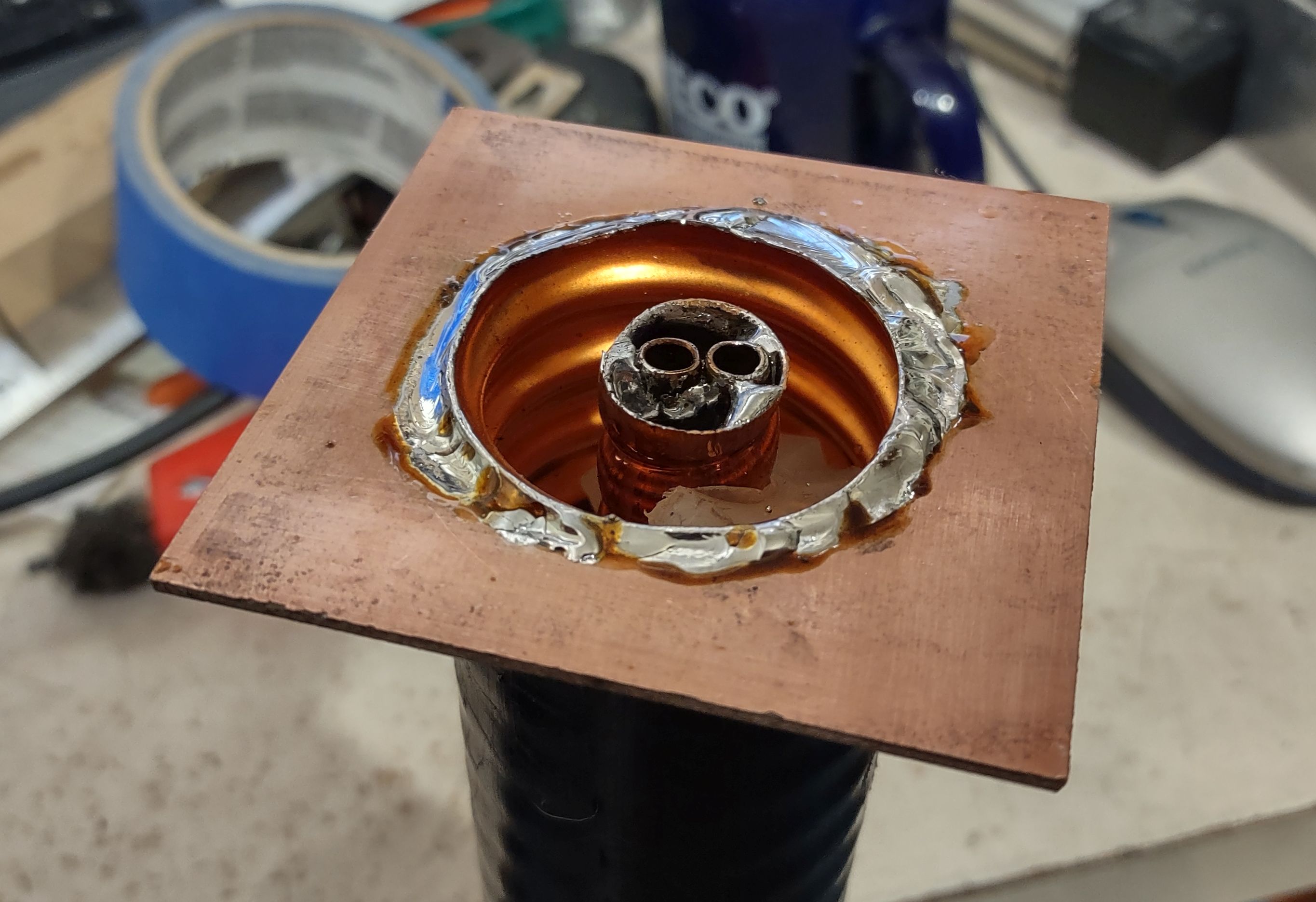
Figure 5:
The "coupling tubes" soldered in place which
receive the wires for coupling in/out.
Click on the image for a larger version.

At this point, the chunk of coax should be trimmed again, measuring from the point where the center conductor is soldered to the shield:  For air-core trim it to 17" (432mm) exactly and for foam core, trim it to 16-1/8" (410mm).  Again, using a sharp knife and gloves, remove about 3/4" (19mm) of the outer jacket and, again, clean the outer conductor so that it is bright and shiny.

Making coupling capacitors:

We now need to make two capacitors to couple the energy from the "in" and "out" connectors to the center resonator and for this, I cut two 3" (75mm) long pieces of RG-6 foam TV coaxial cable and from each of these pieces, I removed and kept the center conductor and dielectric - removing any foil shield and then stripping about 1/2" (12mm) of foam from one end of each piece.

At this point, you'll need some small copper tubing:  I used some 1/4" O.D. soft-drawn tubing, cutting two 2" (50mm) lengths and carefully straightening them out.  To cut this, I used a rotary pipe cutting tool which slightly swedged the ends - but this worked to advantage:  As necessary, I opened up the end cut with the deburring blade of the rotary cutting tool just enough that it allowed the inner dielectric of the RG-6 to slide in and out with a bit of friction to hold it in place..

Comment:

The use of 1/4" (6mm) O.D. copper pipe and RG-6 center conductor/dielectric isn't terribly critical:  A different-sized copper or brass pipe could be used as long as two parallel pieces will fit inside the center conductor of the Heliax - and that the chosen center conductor and dielectric of the coax you use to make the capacitor will fit somewhat snugly inside it.

The reason for the two copper tubes is to prevent the two capacitors made from the center of the RG-6 from coupling directly to each other as all energy must first resonate the center conductor and using these tubes - soldered to the center conductor/resonator - prevents such direct coupling, and it offers good mechanical stability.

Figure 6:
The PC Board plate soldered to the end of the
coax.
Click on the image for a larger version.

Using a hot soldering iron or gun, solder the two straightened pieces of tubing together, in parallel, making sure that the ends of the tubing that you adjust to snugly fit the outside diameter of the piece of RG-6 are at the same end.  Once this is done, insert the two parallel pieces of tubing inside the Heliax's center conductor and solder them, the ends flush with the end of the center conductor, taking care not to heat them enough that they unsolder from each other:  A pair of sharp needle-nose pliers to hold them in place is helpful in this task.

Making a box:

On the "business" (non-shorted) end of the piece of cable we need to make a simple box with a solid electrical connection to the outer shield to which we can mount the RF connectors with good mechanical stability.  For the 1-5/8" cable, I cut a piece of 0.062" (1.58mm) thick double sided glass-epoxy circuit board material into a square that was 3" (75mm) square and using a ruler, drew lines on it from the opposite corners to form an "X" to find the center.

Using a drill press, I used a 1-3/4" (45mm) hole saw to cut a hole in the middle of this piece of circuit board material, using a sharp utility knife to de-burr the edges and to enlarge it slightly so that it would snugly fit over the outside of the cable shield:  You will want to carefully pick the size of hole saw to fit the cable that you use - and it's best that it be slightly undersized and enlarged with a blade or file than oversized and loose.

Figure 7:
Bottom side of the solder plate showing the
connection to the coax.
Click on the image for a larger version.

After cleaning the outside of the coaxial cable and both sides of the circuit board material, solder it to the (non-shorted) end on both sides of the board, almost flush with just enough of the shield protruding through the top to solder it.  For this, a bit of flux is recommended, using a high-power soldering iron or gun - and it's suggested that it first be "tacked" into place with small solder joints to make sure that it is positioned properly.

When positioning the box, rotate it such that the two "capacitor tubes" that were soldered into the center conductor are parallel with one of the sides of the square - this to allow symmetry to the connectors:  This is depicted in Figure 8 where the left-hand and right-hand tubes (more or less) line up with their respective coaxial connectors.

Adding sides and connectors:

With the base of the box in place, cut four sides, each being 1-3/8" (40mm) wide and two of them being 3" (75mm) long and the other two being 2-1/2" (64mm) long.  First, solder the two long pieces to the top, using the shorter pieces inside to space and center them - and then solder the shorter pieces, forming a five-sided (base plus four sides) box atop the piece of cable. As seen in the photo, the "short" sides are parallel to the two tubes in the center conductor.

Figure 8:
Inside the box with coupling/tuning stubs and lines and
stiffening bar installed.  Note the orientation of the tubes.
Click on the image for a larger version.

As can be seen in the picture, BNC connectors were used as they were convenient, but "N" type, SMA or even UHF connectors could be used - but the use of BNC connectors will be described.

The BNC connectors were mounted on opposite sides of the box, approximately 3/8" to the left of the center line and 3/4" from the bottom.  As can be seen in the photo, the connectors were mounted in the "short" wall of the box such that our "RG-6" capacitors more or less line up with the capacitor tubes.

Now, insert the ends of the RG-6 center conductor into the "capacitor tubes" and, bending the top in an "L" shape, solder the end with the exposed center conductor to the coaxial connectors. 

Also visible in Figure 8 - just to the right of the center conductor - are two pieces of copper strip, each about 3/4" (20mm) wide - one is soldered to the center conductor and the other to the ground inside the box.  These two tabs form a very simple capacitor which may be used to "fine tune" the center frequency of the pass response by bending them nearer/closer to each other.  While most of the adjustment of the center tuning will occur as one slides the two capacitors (made from RG-6) in and out, this method may also be used to provide a bit of additional tuning range.

Preliminary adjustment:

It is best to first set the RG-6 capacitors to obtain the desired pass response, taking into account the desired band-pass frequency, but once one has done this - and if the pass frequency is too high - one would then add the "copper tab" capacitors - perhaps more than one set.  If the frequency is too low, see if you can obtain a suitable passband width (and acceptable insertion loss) by pulling these coupling capacitors out to raise the frequency:  For most applications, an insertion loss of even 1 dB will not appreciably reduce receiver performance - particularly if the local noise at the site is rather high from other users and especially if the use of a band-pass filter like this is intended to minimize desense, anyway.

It is best to make them from metal (copper, brass) that is thick enough to not be springy on their own:  Saving a piece and flattening the copper material from the shield of the 1-5/8" coax as you prepare it for use is suggested.

At this point we are ready to do some preliminary tuning - and this will require a NanoVNA or similar:  It is presumed that the builder will have familiarity with the NanoVNA to make S11 VSWR and S12 insertion loss measurements on an instrument that has been properly calibrated at the frequency range in question.

Setting the NanoVNA to measure both VSWR and through-loss over a span of 130-160 MHz, connect it to the cable and you should see a pass response somewhere in the frequency range and if all goes well, the peak in the pass response will be somewhere in the 130-140 MHz range.

Adjusting the center frequency and passband response is an iterative process as reducing the coupling by pulling out the capacitors (the RG-6 center conductor) will also increase the frequency.  Practically speaking, only about 3/8"-1/2" (9-12mm) of center conductor is needed at most to attain optimal coupling so don't be afraid to pull out more and more of the capacitors.

A bit of experimentation is suggested here to get the "feel" of the adjustment - and here are a few pointers:

• 

  Figure 9:
  The band-pass filter sitting against a Sinclair
  Q2220E 2-meter Duplexer - a good combination
  for receiver protection at a busy repeater site!
  Click on the image for a larger version.
  

  Lowest SWR is obtained with the coupling capacitors are identically adjusted.  If the SWR isn't below 1.5:1, try pulling out or pushing in one of the capacitors slightly to determine the effect - but move it only about 1/16" in each iteration.  Generally speaking, pulling one out slightly is the same as pushing the other in slightly in terms of reducing VSWR.
• The passband response will be narrower the less of the RG-6 center conductor is in the capacitor tubes - but the insertion loss will also go up.
  
• The frequency will go up the more the passband response is narrowed by reducing the coupling capacitors.
• With the lengths given (e.g. 17" for air-core 16-1/8" for foam core) the passband will be within the 2 meter band with the amount of coupling that will yield about 0.5-0.6 dB insertion loss.  To a degree, you can "tune" the center frequency of the cavity by adjusting the coupling.  It is recommended that you first tune for the bandpass response - and then tune it to frequency: See below for additional comments.
  
• It is recommended that you use a little coupling as needed to obtain the desired response.  For example, if the cavity is "over coupled", the insertion loss will be about 0.5dB, but this will go up only very slightly as the coupling is reduced and the response is narrowed.  At some point the insertion loss will start to go up as the passband is further-narrowed.
• As the coupling capacitor is pushed in, the resonant frequency will go down.  If, even with the "tuning capacitor" (the copper strips) are minimized in coupling,  the frequency is too low, try pulling the RG-6 capacitors out slightly to move it up in frequency:  It's easy to accidentally "over couple" the cavity by pushing them in too far and causing it to tune low.   It's likely that you can pull more of the RG-6 capacitors out and reducing coupling than you might first think and still have acceptably-low insertion loss - and doing so will narrow the passband response and improve ultimate off-frequency attenuation.
  

As mentioned above, it's recommended that the approximate passband width be set with the capacitors and if all goes well, the pass frequency can be adjusted with just the adjustment to the coupling with only a slight change in overall bandwidth.  If, however, the desired "narrowness" results in a pass frequency above that which is desired, a simple "tab" capacitor can be constructed as shown in the photo.

Figure 10:
The "close-in" response of the band-pass cavity.
With the current settings providing a bit less than 0.5dB of
attenuation at the center, it's rejection at the edges of the
U.S. 2 meter band (144-148 MHz) is a bit over 8 dB.
Click on the image for a larger version.

This capacitor consists of two parts:  A 3/8" (10mm) wide, 3/4" (20mm) long piece of copper or brass sheet is soldered to the center conductor.  The addition of this piece, alone, may lower the center frequency and bending this tab up and down can provide a degree of fine-tuning.  If the center frequency is still too high, another 3/8" wide, 3/4" long piece can be soldered to the shield of the coax next to it and be bent such that it and the first piece form two plates of a simple capacitor, allowing even greater reducing in resonant frequency of the cavity.

With the preliminary tuning done, a bit of reinforcement of the box is suggested:  A strip of copper circuit board material 3/8"-1/2" (9-12nn) wide is soldered between the inside walls of the box with the RF connectors.  This strip minimizes the flexing of the walls with the RF connectors due to stresses on the connected cables which can change the orientation of the coupling capacitors and cause slight detuning.

With this reinforcement in place, do a final tweaking of the bandpass filter's tuning.

Final assembly:

As noted earlier, it's strongly suggested that the shorted end of the cavity be covered to prevent debris and insects from entering either the center conductor or, especially, the space between the shield and center conductor.  This may be done using electrical tape or RTV (Silicone) adhesive.

Figure 11:
A wider sweep showing the rejection at and below the FM
broadcast band and up through 225 MHz.  This
filter, by itself, provides over 40 dB rejection at 108 MHz
Click on the image for a larger version.

Similar protection should be done to the top of the box:  A piece of brass or copper sheet - or a piece of PC board material could be tack-soldered into place - or even some aluminum foil tape could be used:  The tuning should be barely affected - if at all - by the addition of this cover, but it is worth verifying this with a simple test-fit of the cover.

Additional comments:

While the performance will vary depending on the coupling and tuning, the prototype, tuned for a pass response at 146.0 MHz, performed as follows:

• Insertion loss at resonance:  <0.5dB
• -3dB points:  -88 kHz and +92 kHz
  
• -10dB points:  -2.5 MHz and +2.75 MHz
• -20dB points:  -7.6 MHz and +11 MHz
• 2:1 VSWR bandwidth:  600 kHz
• Loss <=108 MHz:  40dB or greater

More detail about the response of this cavity filter may be seen in figures 10 and 11.  In the upper-left corner of each figure may be found the measured loss and VSWR at each of the on-screen markers.

If a higher insertion loss can be tolerated, the measured bandwidths will be narrower.  Depending on the situation, an extra dB or two of path loss may be a reasonable trade-off for improved off-frequency rejection - particularly on a noisy site where the extra loss won't result in a degradation of system sensitivity due to the elevated noise floor.

As with any cavity-type filter, there is a bit of fragility in terms of frequency stability with handling.  If, after it is tuned this - or any cavity filter - is dropped or jarred strongly, the tuning should be re-checked and adjusted as necessary.

There's no reason why this cavity couldn't be used for transmitting, although using the materials described (e.g. the center conductors of RG-6) I would limit the power to 10-15 watts without additional testing.

As it is, this band-pass filter - in conjunction with a conventional 2-meter duplexer - can provide a significant reduction in off-frequency energy that could degrade receiver performance.  As can be seen in Figure 2, the pass cavity may still pass energy from odd-order (3rd, 5th) harmonics that may fall within commercial/70cm and TV broadcast frequencies - but the addition of a VHF low-pass filter - perhaps even the VHF side of a VHF/UHF mobile diplexer - would eliminate these responses.

To be a good neighbor on a busy site it's strongly recommended that a pass cavity also be installed on the transmit side, along with a ferrite isolator (e.g. circulator with dummy load) to deal with signals that may enter into the transmitter's output stage and mix, causing intermodulation distortion and interference - both to your own receiver and those of others. 

* * * * * * 

Specific use cases:

Reduction of ingress from FM broadcast transmitters:

The most obvious use case would be the filtering of co-located FM broadcast transmitters.  Despite being about 50 MHz off-frequency, a nearby FM transmitter - which often runs hundreds if not thousands of watts - can couple into a 2 meter antenna with sufficient energy to overload a receiver, causing the appearance of distorted audio from the wideband FM modulation of the broadcast transmitter to appear on the receiver.  I have been on sites where the measured power at the receiver terminals, after passing through the 2 meter duplexer, have been on the order of 10 to 20 dBm (10-100 milliwatts) and actually registered as reflected power on an SWR bridge.

As can be seen from the above graphs and measurement, the filter described is capable of reducing this signal by at least 40 dB - likely enough to prevent gross overload of the receiver in question.

Reduction of commercial high-band VHF signals:

While less common these days, there are still systems like community repeaters operating above the 2 meter band in the 150-170 MHz range.  These, too, can cause receiver degradation and the fact that these signals may be intermittent (e.g. a repeater that isn't used too often) can often frustrate the analysis of intermittent "desense" issues.  Even this humble cavity is capable of reducing such a signal by about 20 dB at and above 155 MHz - more, if one were to reduce the coupling (and response bandwidth) of the cavity:  In severe cases, the slightly higher insertion loss of the filter (say, 1.5 dB instead of less than 0.5 dB) may well be worth the trade-off in off-frequency rejection.

* * * * * *

"I have 'xxx' type of cable - will it work?"

The dimensions given in this article are approximate, but should be "close-ish" for most types of air and foam dielectric cable.  While I have not constructed a band-pass filter with much smaller cable like 1/2" or 3/4", it should work - but one should expect somewhat lower performance (e.g. not-as-narrow band-pass with higher losses) - but it may still be useful.

Because of the wide availability of tools like the NanoVNA, constructing this sort of device is made much easier and allows one to characterize both its insertion loss and response as well as experimentally determining what is required to use whatever large-ish coaxial cable that you might have on-hand.

* * * * * *

Future article: 

I have constructed several effective notch-type cavities from this type of coaxial cable - including one that is designed to attenuate 144.39 MHz APRS energy in a 147 MHz repeater's receiver - but since there are relatively few articles about pass-type cavities constructed in this way, I decided to post this one first.

Related articles:

• Second Generation Six-Meter Heliax Duplexer by KF6YB - link  - This article describes a notch type duplexer rather than pass cavities, but the concerns and construction techniques are similar.
  

• When Band-Pass/Band-Reject (Bp/Br) Duplexers really aren't bandpass - link - This is a longer, more in-depth discussion about the issues with such devices and why pass cavities should be important components in any repeater system.

 

This article was stolen from ka7oei.blogspot.com

[END]