A 173 mile (278km) all-electronics, FSO (Free Space Optical) contact: Part 1 - Scouting it out

Nearly 10 years ago - in October, 2007, to be precise - we (exactly "who" to be mentioned later) successfully managed a 173 mile, Earth-based all-electronic two-way contact between two remote mountain ranges in western Utah.

For many years before this I'd been mulling over in the back of my mind various ways that optical ("lightbeam") communications could be accomplished over long distances.  Years ago, I'd observed that even a modest, 2 AA-cell focused-beam flashlight could be easily seen over a distance of more than 30 miles (50km) and that sighting even the lowest-power Laser over similar distances was fairly trivial - even if holding a steady beam was not.  Other than keeping such ideas in the back of my head, I never really did more that this - at least until the summer of 2006, when I ran across a web site that intrigued me, the "Modulated Light DX page" written by Chris Long (now amateur radio operator VK3AML) and Dr. Mike Groth (VK7MJ).  While I'd been following the history and progress of such things all along, this and similar pages rekindled the intrigue, causing me to do additional research - and I began to build things.

Working up to the distance...

Over the winter of 2006-2007 I spent some time building, refining, and rebuilding various circuits having to do with optical communications.  Of particular interest to me were circuits used for detecting weak optical signals and it was those that I wanted to see if I could improve.  After considerable experimentation, head-scratching, cogitation, and testing, I was finally able to come up with a fairly simple optical receiver circuit that was at least 10dB more sensitive than other voice-bandwidth circuits that were out there.  Other experimentation was done on modulating light sources and the first serious attempt at this was building a PIC-based PWM (Pulse-Width Modulation) circuit followed, somewhat later, by a simpler current-linear modulator - both being approaches that seemed to work extremely well.

After this came the hard part:  Actually assembling the mechanical parts that made up the optical transceivers.  I decided to follow the field-proven Australian approach of using large, plastic, molded Fresnel lenses in conjunction with high-power LEDs for the source of light emissions with a second parallel lens and a photodiode for reception and the stated reasons for taking this approach seemed to me to be quite well thought-out and sound - both technically and practically.  This led to the eventual construction of an optical transceiver that consisted of a pair of identical Fresnel lenses, each being 318 x 250mm (12.5" x 9.8") mounted side-by-side in a rigid, wooden enclosure comprising an optical transceiver with parallel transmit and receive "beams."  In taking this approach, proper aiming of either the transmitter or receiver would guarantee that the other was already aimed - or very close to being properly aimed - requiring only a single piece of gear to be deployed with precision.

After completing this first transceiver I hastily built a second transceiver to be used at the "other" end of test path.  Constructed of foam-core posterboard, picture frames and inexpensive, flexible vinyl "full-page" magnifier Fresnel lenses, this transceiver used, for the optical emitter and transmitter assemblies, my original, roughly-repackaged prototype circuits.  While it was neither pretty or capable of particularly high performance, it filled the need of being the "other" unit with which communications could be carried out for testing:  After all, what good would a receiver be if there were no transmitters?

On March 31, 2007 we completed our first 2-way optical QSO with a path that crossed the Salt Lake Valley, a distance of about 24 km (15 miles.)  We were pleased to note that our signals were extremely strong and, despite the fact that our optical path crossed directly over downtown Salt Lake City, they seemed to have 30-40dB signal-noise ratio - if you ignored some 120 Hz hum and the occasional "buzz" from an unseen, failing streetlight.  We also noted a fair amount of amplitude scintillation, but this wasn't too surprising considering that the streetlights visible from our locations also seemed to shimmer being subject to the turbulence caused by the ever-present temperature inversion layer in the valley.

Bolstered by this success we conducted several other experiments over the next several months, continuing to improve and build more gear, gain experience, and refine our techniques.  Finally, for August 18, 2007, we decided on a more ambitious goal:  The spanning of a 107-mile optical path.  By this time, I'd completed a third optical transceiver using a pair of larger (430mm x 404mm, or 16.9" x 15.9") Fresnel lenses, and it significantly out-performed the "posterboard" version that had been used earlier.  On this occasion we were dismayed by the amount of haze in the air - the remnants of smoke that had blown into the area just that day from California wildfires.  Ron, K7RJ and company (his wife Elaine, N7BDZ and Gordon, K7HFV) who went to the northern end of the path (near Willard Peak, north of Ogden, Utah) experienced even more trials, having had to retreat on three occasions from their chosen vantage point due to brief, but intense thunderstorms.  Finally, just before midnight, a voice exchange was completed with some difficulty - despite the fact that they never could see the distant transmitter with the naked eye due to the combination of haze and light pollution - over this path, with the southern end (with Clint, KA7OEI and Tom, W7ETR) located near Mount Nebo, southeast of Payson, Utah.

Figure 1:
The predicted path projected onto a combination
map and satellite image.  At the south end
(bottom) is Swasey Peak while George Peak is
indicated at the north.
Click on the image for a larger version.

Finding a longer path:


Following the successful 107-mile exchange we decided that it was time to try an even-greater distance.  After staring at maps and poring over topographical data we found what we believed to be a 173-mile line-of-sight shot that seemed to provide reasonable accessibility at both ends - see figure 1.  This path spanned the Great Salt Lake Desert - some of the flattest, desolate, and most remote land in the continental U.S.  At the south end of this path was Swasey Peak, the tallest point in the House range, a series of mountains about 70 miles west of Delta, in west-central Utah.  Because Gordon had hiked this peak on more than one occasion we were confident that this goal was quite attainable.

At the north end of the path was George Peak in the Raft River range, an obscure line of mountains that run east and west in the extreme northwest corner of Utah, just south of the Idaho boarder.  None of us had ever been there before, but our research indicated that it should be possible to drive there using a high-clearance 4-wheel drive vehicle so, on August 25, 2007, Ron and Gordon piled into my Jeep (along with a 2^nd spare tire swiped from Ron's Jeep as recommended by more than one account) and we headed north to investigate.

Getting there:

Following the Interstate highway nearly to the Idaho border, we turned west onto a state highway, following it as the road swung north into Idaho, passing the Raft River range, and we then turned off onto a gravel road to Standrod, Utah.  In this small town (a spread-out collection of houses, really) we turned onto a county road that began to take us up canyons on the northern slope of the range.  As we continued to climb, the road became rougher and we resorted to peering at maps and using our intuition to guide us onto the one road that would take us to the top of the mountain range.

Luckily, our guesses were correct and we soon found ourselves at the top of the ridge.  Traveling for a short distance, we ran into a problem:  The road stopped at a fence gate that was plastered with "No Trespassing" signs.  At this point, we simply began to follow what looked like road that paralleled the fence only to discover, after traveling several hundred feet - and past a point at which we could safely turn around - that this "road" had degenerated into a rather precarious dirt path traversing a steep slope.  After driving several hundred more feet, fighting all the while to keep the Jeep on the road and moving in a generally forward direction, the path leveled out once again and rejoined what appeared to be the main road.  After a combination of both swearing at and praising deities we vowed that we would never travel on that "road" again and simply stay on what had appeared to have been the main road, regardless of what the signs on the gates said!

Looking for Swasey Peak:

Having passed these trials, we drove along the range's ridge top, looking to the south.  On this day, the air was quite hazy - probably due to wildfires that were burning in California, and in the distance we could vaguely spot, with our naked eyes, the outline of a mountain range that we thought to be the House range:  In comparing its outline and position with a computer-simulated view, it "looked" to be a fairly close match as best as we could guess.

Upon seeing this distant mountain we stopped to get a better look, but when we looked through binoculars or a telescope the distant outline seemed to disappear - only to reappear once again when viewed with the naked eye.  We finally realized what was happening:  Our eyes and brain are "wired" to look at objects, in part, by detecting their outlines, but in this case the haze reduced the contrast considerably.  With the naked eye, the distant mountain was quite small but with the enlarged image in the binoculars and telescope the apparent contrast gradient around the object's outline was greatly diminished.  The trick to being able to visualize the distant mountain turned out be keeping the binoculars moving as our eyes and brain are much more sensitive to slight changes in brightness of moving objects than stationary ones.  After discovering this fact, we noticed with some amusement that the distant mountain seemed to vanish from sight once we stopped wiggling the binoculars only to magically reappear when we moved them again.  For later analysis we also took pictures at this same location and noted the GPS coordinates.

Continuing onwards, we drove along the ridge toward George Peak.  When we got near the GPS coordinates that I had marked for the peak we were somewhat disappointed - but not surprised:  The highest spot in the neighborhood, the peak, was one of several gentle, nondescript hills that rose above the road only by a few 10's of feet.  Stopping, we ate lunch, looked through binoculars and telescopes, took pictures, recorded GPS coordinates, and thought apprehensively about the return trip along the road.

Figure 2:
The predicted line-of-sight view (top) based on 1 arc-second SRTM terrain data between the Raft River range
and Swasey peak as seen from the north (Raft River) side.
On the bottom is an actual photograph of the same scene at the location used in the simulated view.  As can be seen,
more of the distant mountain can be seen than the prediction would indicate, this being due to the refraction of
the atmosphere slightly extending the visible horizon.  Under typical conditions, this "extension" amounts to
an increase of approximately 10/9th of the distance than geometry would predict.  This lower picture was produced
by "stacking" multiple images using software designed for astronomy.
Click on the image for a larger version.

Returning home:

Retracing our path - but not taking the "road" that had paralleled the fence line - we soon came to the gate that marked the boundary of the private land.  While many of the markings were the same at this gate, we noticed another sign - one that had been missing from the other end of the road - indicating that this was, in fact, a public right-of-way plus the admonition that those traveling through must stay on the road.  This sign seemed to register with what we thought we'd remembered about Utah laws governing the use of such roads and our initial interpretation of the county parcel maps:  Always leave a gate the way you found it, and don't go off the road!  With relief, we crossed this parcel with no difficulty and soon found ourselves at the other gate and in familiar territory.

Retracing our steps down the mountain we found ourselves hurtling along the state highway a bit more than an hour later - until I heard the unwelcome sound of a noisy tire.  Quickly pulling over I discovered that a large rock that had embedded itself in the middle of the tread of a rear tire.  After 45 minutes of changing the tire and bringing the spare up to full pressure, we were again underway - but with only one spare remaining...

Analyzing the path:

Upon returning home I was able to analyze the photographs that I had taken.  Fortunately, my digital SLR camera takes pictures in "Raw" image mode, preserving the digital picture without loss caused by converting it to a lossy format like JPEG.  Through considerable contrast enhancement, the "stacking" of several similar images using an astronomical photo processing program and making a comparison against computer-generated view I discovered that the faint outline that we'd seen was not Swasey Peak but was, in fact, a range that was about 25 miles (40km) closer - the Fish Springs mountains - a mere 150 or so miles (240km) away.  Unnoticed (or invisible) at the time of our mountaintop visit was another small bump in the distance that was, in fact, Swasey Peak.

Interestingly, the first set of pictures were taken at a location that, according to the computer analysis, was barely line-of-sight with Swasey Peak.  At the time of the site visit we had assumed that the just-visible mountain that we'd seen in the distance was Swasey Peak and that there was some sort of parallax error in the computer simulation, but analysis revealed that not only was the computer simulation correct in its positioning of the distant features, but also that the apparent height of Swasey Peak above the horizon was being enhanced by atmospheric refraction - a property that the program did not take into account:  Figure 2 shows a comparison between the computer simulation and an actual photograph taken from this same location.


Building confidence - A retry of the 107-mile path:

Having verified to our satisfaction that we could not only get to the top of the Raft River mountains, but also that we also had a line-of-sight path to Swasey Peak, we began to plan for our next adventure.  Over the next several weeks we watched the weather and the air - but before we did this, we wanted to try our 107-mile path again in clearer weather to make sure that our gear was working, to gain more experience with its setup and operation, and to see how well it would work over a long optical path given reasonably good seeing conditions:  If we had good success over a 107-mile path we felt confident that we should be able to manage a 173-mile path.

A few weeks later, on September 3, we got our chance:  Taking advantage of clear weather just after a storm front had moved through the area we went back to our respective locations - Ron, Gordon and Elaine at Inspiration Point while I went (with Dale, WB7FID) back to the location near Mt. Nebo.  This time, signal-to-noise ratios were 26dB better than before and voice was "armchair" copy.  Over the several hours of experimentation we were able to transmit not only voice, but SSTV (Slow-Scan Television) images over the LED link - even switching over to using a "raw" Laser Pointer for one experiment and a Laser module collimated by an 8" reflector telescope in another.

With our success on the clear-weather 107-mile path we waited for our window to attempt the 173-mile path between Swasey and George Peak but in the following weeks we were dismayed by the appearance of bad weather and/or frequent haze - some of the latter resulting from the still-burning wildfires around the western U.S.

To be continued!

[End]

This page was stolen from "ka7oei.blogspot.com"

A daylight-tolerant TIA (TransImpedance Amplifier) optical receiver

While the majority of my past experiments with through-the-air free-space optical (FSO) communications were done at night, for obvious reasons, I had also dabbled in optical communications done during broad daylight, with and without clouds.

The challenge of daylight:

Clearly, the use of the cloak of darkness has tremendous advantages in terms of signal-noise ratio and practically-attainable communications distances, but daylight free-space optical communications has some interesting aspects of its own:

• It's easier to see what you are doing, since it's daylight!
• Landmarks are often easier to spot, aiding the aiming.
• Even in broad daylight, it is possible to provide signaling as an aiming aid, such as a mirror reflecting the sun - assuming that it is sunny.
• The sun is a tremendous source of thermal noise, causing dilution of the desired signals.
• Great care must be taken when one wields optics during the day:  Pointing at the sun or a very strong specular reflection - even briefly - can destroy electronics or even set fire to various parts of the lens assembly!

As you might expect the biggest limitation to range is the fact that the sun, with its irradiance of around 1kW/m³ (when sunny) can overwhelm practically any other source:  This is why the earliest "wireless" communications methods often used reflected sunlight, notably the Heliograph, where a mirror was "modulated" with telegraph code, or the "Photophone", a wireless audio transmitter using reflected light, an invention of Alexander Graham Bell from the 1870s with earlier roots - a device that Bell himself considered to be his greatest invention.

Figure 1:
Optical communications during daylight.  In the center of this contrast-enhanced picture (the red spot) is the light from an optical transmitter using a 30+ watt LED at a distance of 13.25 miles (21.3km).  This image is from my own "modulatedlight" web site.
Click on the image for a larger version.

Means of detection:

While the modulated speech may be produced in any number of ways (vibrating mirror, high-power LED, LASER) some thought must be given on the subject of how to detect it.  While the detector itself need not be spectacularly sensitive due to the nearly overwhelming presence of the thermal noise from the sun, it is worth making it "reasonably" sensitive so that this is not the limiting factor.  An example of an un-sensitive optical receiver (e.g. one that is rather "deaf" and itself is not likely to be sensitive enough even for daylight use) is a simple circuit using a phototransistor as depicted below:

Figure 2:
A simple phototransistor-based receiver (top):  Note that there's an error in the diagram in that it shows a photodiode instead of a phototransistor.  This circuit was built by Ron, K7RJ, simply to demonstrate the ability to convey audio a short distance:  It is (intentionally) not optimized in any way and is not at all sensitive!  A similar, but slightly better circuit was found on the Ramsey Electronics LBC6K "Laser Communicator", which was also quite "deaf".  See the article Using Laser Pointers for Free-Space Optical Communications - link that more thoroughly explains this issue.  This image is from my own "modulatedlight.org" web site and used with the permission of Ron Jones, K7RJ.
Click on the image for a larger version.

The circuit in the top half of Figure 2 (above) depicts one of the simplest-possible optical receivers - and one of the "deafer" options out there.  In this case a biased phototransistor is simply fed into an LM386 audio amplifier and the signal is amplified some 200-fold (about 46dB.)  As noted in the caption, this was a "quick and dirty" circuit to prove a concept and was, by no means optimized nor does it take maximum advantage of the potential performance of a detector.

As it turns out a phototransistor isn't really the ideal device because it is, by itself, intrinsically noisy.  Another, more practical issue is that its active area is typically quite small which means that it won't intercept much light on its own.  Of course, any half-hearted attempt to use any device for the detection of optical signals over even a rather short distance of a few hundred meters would include the use of a lens in front of the detector - no matter its type:  The lens will easily increase the "capture area" by many hundred-fold (even for a small lens!) and will effect noiseless amplification with the added benefit of rejecting light sources that are off-axis.  With the tiny active area of a phototransistor it can be difficult to properly and precisely focus the distant light onto that area and it is likely that unless very good precision in both alignment and focus can be maintained, the "spot of light" being focused onto the phototransistor will be larger than its active area, "wasting" some of its light as it "spill"s over the sides.

One of the biggest problems with a circuit like this is that there will be a level of light at which the phototransistor saturates, and when this happens the voltage across its collector and emitter will go very close to zero and the received signals will disappear, possibly "un-saturating" only briefly during those points in the modulation where the source light happens to go toward zero, resulting in badly distorted sound.  In broad daylight the phototransistor may be hopelessly saturated at all times unless an optical attenuator (e.g. neutral density filter) is used to reduce the total light level and/or more current is forced through it.

Introducing the TransImpedance Amplifier (TIA):

A much better circuit is the TransImpedance Amplifier, a simple circuit that proportionally converts current to voltage.  With this circuit (see Figure 3) one would more likely use a PIN Photodiode, a device akin to a solar cell, in which the output current is pretty much proportional to the light hitting its active area. This is quite unlike the manner in which a phototransistor is typically used where in the former case the impinging light causes a voltage drop across the device.

Figure 3:
A simple transimpedance amplifier.
(Image from Wikipedia)

In this circuit the junction between the inverting (-) and noninverting (+) inputs of the op-amp "wants" to be zero, so as the current from the photodiode increases in the presence of light, its output voltage will increase, sending a portion of that current through feedback resistor "Rf" until the overall voltage is zero.  What this means is that the output voltage, Vout, is equal to the current in the photodiode multiplied by the magnitude of resistance, Rf - except that the voltage will be negative, since this is an inverting amplifier.

As an example, assume that Rf is set to 1 Megohm.  Assuming no leakage and a "perfect" op-amp we can determine that if there is -1 volt output, we must have 1/1000000^th of an amp (e.g. 1 microamp) attributed to Ip, the photodiode current.  This sort of circuit is often used as a radiometric detector - that is one in which its output is directly proportional to the amount of light striking the photodiode' surface, weighted by intervening optics and filters and the spectral response of the detector itself.

For more about the Transimpedance Amplifier circuit, visit the Wikipedia page on the subject - link.

This is OK when the photodiode is in complete darkness - or in near-complete darkness, but what about strong light?  We can see from the above example that if we have just 10 microamps - a perfectly reasonable value for a typical photodiode such as the BPW34 in dim-to-normal room lighting - that Vout would be -10 volts.  If this same circuit were taken outside, the diode current could well be many hundreds or thousands of times that amount and this would "slam" the output of the op amp against a power supply rail.

A daylight-tolerant TIA:

One of the typical means of counteracting this effect is to capacitively couple the photodiode to the op amp so that only changing currents from a modulated signal get coupled to it, blocking the DC, but there is another circuit that is arguably more effective, depicted in Figure 4, below.

Figure 4:
A "Daylight Tolerant" Transimpedance amplifier circuit.
In this circuit the DC from the output is fed back to "servo" the photodiode's "cold" side so that its "hot" side (that connected to the op amp's inverting input) is always maintained at the same potential as the noninverting input, eliminating the DC offset caused by ambient light.  The disadvantage of this method is that it does not lend itself well to reverse-biasing the photodiode to reduce its capacitance, but between the high intrinsic thermal noise levels of daylight and the related photoconductive shunting of the device due to high ambient light, this is largely unimportant.  For the photodiode the common and inexpensive BPW34 may be used along with many other similar devices.
Click on the image for a larger version.

This circuit is, at its base, the same as that depicted in Figure 3, with a few key differences:

• An "artificial ground" is established using R101 and R102, allowing the use of a single-polarity power supply.  This artificial ground is coupled to the actual ground via C102 and C103 making it low impedance to all but DC and very low AC frequencies.
• The voltage output from the transimpedance amplifier section (U101a) is feed back via R104 to the "ground" side of the photodiode (D101) to change its "ground".  If there is a high level of ambient light, the voltage at the "bottom" end of D101 (at D101/C107) goes negative with respect to the artificial ground, setting the DC voltage at the non-inverting input of the op amp to zero, cancelling it out.
• R104 and C106 form a low-pass filter that passes the DC offset voltage to the bottom of D101, but blocks the audio.  In this way the DC resulting from ambient light that would "slam" the op amp's output to the negative rail is cancelled out, but the AC (audio) signals remain.  The time constant of this R/C network is slow enough to be "invisible" all but the very lowest (subaudible) frequencies, but more than fast enough to track changes in ambient light.
• By not placing any additional components between the "hot" end of the photodiode and the op amp, the introduction of additional noise from the components (including microphonic responses of the coupling capacitor) is greatly reduced.

In the above circuit the values of R103 and C104 would be chosen for the specific application.  In a circuit that is to be used at very high light levels where high sensitivity is not very important a typical value of R103 would be 100k to 1 Megohm:  Do not use a carbon composition but a carbon film or (better yet) metal film resistor is preferred for reasons of noise contribution.  While tempting to use, a variable resistor at R103 is also not recommended as these can be a significant source of noise.  If multiple gain ranges are used, small DIP switches, push-on jumpers or even high-quality relays - wired to the circuit - could be used to select different feedback resistances, knowing that these devices have the potential of introducing noise as well as additional stray circuit capacitance.  (Such a relay/switch would be wired on the "output" side of the op amp/relay of the feedback resistance(s) and proper component selection, layout and appropriate shielding would need to be considered.)

C104 is used to compensate for photodiode and other circuit capacitance and without it the high frequency components would rise up (e.g. "peak"), possibly resulting in oscillation and general instability.  Typical values for C104 when using a small-ish photodiode like the BPW34 are 2-10pF:  Using too much capacitance will result in unnecessarily rolling off high frequency components, but will not otherwise cause any problems.  A small trimmer capacitor may be used for C104, either "dialed in" for the desired response and left in permanently or optimally adjusted, measured, and then replaced with an equal-value fixed unit.

Again, the reason why the ultimate in high sensitivity is not required on a "Daylight Tolerant" circuit is that during the daytime, the dominant signal will be due to thermal noise from the sun - a signal source strong enough that it will submerge weak signals, anyway:  It need be sensitive enough only to be able to detect the sun noise during daylight hours.

The op amp noted in Figure 4 is the venerable LM833, a reasonably low-noise amplifier and one that is cheap and readily available (and actually works well down to 7 volts - a bit below its "official" voltage rating allowing the above circuit to powered from a single 9 volt battery) but practically any decent low-noise op amp could be used:  Somewhat better performance may be obtained using special, low-noise op amps, but these would be "overkill" under daylight conditions.

For nighttime use - where better sensitivity was important - a standard "TIA" amplifier that omits the DC feedback loop to cancel out the DC (potentially noise-contributing) components along with higher values of Rf would offer better performance, but for much better low-noise performance (e.g. 10-20dB better ultimate sensitivity) under low-light conditions than is possible with standard components at audio frequencies in a TIA configuration the "Version 3" optical receiver circuit described on the page "Gate Current in a JFET..." - link is recommended, instead.


Additional web pages on related topics:

• Daylight Optical Experimentation -  This page describes experiments done in broad daylight over 13 mile (21km) free-space links.
  
• Modulatedlight.org - This web site has a wide variety of information related to amateur, free-space optical, through-the-air communications.
• Optical Receivers for Low-Bandwidth, Through-the-Air Communications - This is a reference article that gives additional detail about the design of the circuits discussed in this article.
• Using Laser Pointers for Free-Space Optical Communications - This describes how one might use low-power laser pointers for low-rate optical communications, the practicalities of various circuits, the methods and the realities.
• The Modulated Light DX page - This page has several articles describing the practical aspects of free-space, through-the-air optical communications including various atmospheric effects.

The above web pages also contain links to other, related pages on similar subjects.


[End]

This page stolen from "ka7oei.blogspot.com".

Combatting scintillation effects on optical voice links

One interesting aspect of the amateur radio hobby that is rarely discussed is the use of the "Above 275 GHz" bands.  While one might, at first, think that this might require some exotic "componentry" to use these wavelengths, to assume such would ignore the fact that this includes "optical" frequencies - which is to say, visible light.

Working with visible light has a tremendous advantage over other "frequencies" in that we have some built-in test equipment:  Our eyes.  While generally uncalibrated in terms of "frequency" and power (e.g. brightness) they are of great help in building, setting up and troubleshooting such equipment.

For years now lasers have been considered to be the primary source of optical transmitters - which makes sense for some of the following reasons:

• Lasers are cool!
• They may be easily modulated.
• Lasers are cool!
• "Out of the box" they produce nicely collimated beams.
• Lasers are cool!
• Low-power diode-based lasers are inexpensive and easy to use.
• Lasers are cool!

While lasers are (almost) exclusively used for all types of fiber-optic based communications, one might ask oneself if they are equally useful/effective when the medium is the atmosphere rather than a stable, glass conduit?

The answer is:  It depends.

If one is going very short distances - perhaps up to a few hundred meters - the atmosphere can be largely ignored unless there is something that is causing severe attenuation of the signals (e.g. rain, snow or fog) but as the distances increase - even if there is not some sort of adverse condition causing such loss - there are typically nonuniformities in the atmosphere caused by thermal discontinuities, wind, atmospheric particulates, etc. that causes additional disruption.

The fact that Lasers produce (generally) coherent beams in terms of frequency and phase - gas lasers usually more so than most semiconductor types - actually works against efforts in making a long-distance, viable communications link because the atmosphere causes phase disruptions along the path length resulting in rapid changes in amplitude due to both constructive and destructive interference of the wavefront.

In the past decade or so, high-power LEDs have become available with significant optical flux.  Unlike Lasers, LEDs do not produce a coherent wavefront and because of this they are generally less affected by such atmospheric phenomenon, as the video below demonstrates:

Figure 1:

Visual example of laser versus LED "lightbeam"

communications.

Admittedly, the example depicted in Figure 1 is somewhat unfair:  The transmit aperture of the laser used for this test was very small, a cross-sectional area of, perhaps, 3-10 square millimeters, while the aperture of the LED optical transmitter was on the order of 500 square centimeters.  Even if both light sources were of equal quality and type (e.g. both laser or both LED) that using the smaller-sized aperture would be at a disadvantage due to the lack of "aperture averaging" - that is, more subject to scintillation due to the small, angular size of the beam causing what is sometimes referred to as "local coherence" where even white light can, for brief, random intervals, take on the interference properties of coherent light:  It is this phenomenon that causes stars to twinkle - even briefly change color - while astronomical objects of larger apparent size such as planets usually do not twinkle.

Figure 2:
Adapter used for emission of laser light via the telescope.
Contained within is a laser diode modified to produce
a broad, fan pattern to illuminate the mirror of the
telescope.

For an interesting article on the subject of scintillation, see "The Sizes of Stars" by Calvert - LINK.

Based on this one might conclude that the larger the aperture for emitting will reduce the likelihood that the overall beam will be disrupted by atmospheric effects - and one would be correct.  The use of a large-area aperture tends to reduce the degree of "local coherence" described in the Calvert article (linked above) while also providing a degree of "aperture averaging".  As an aside, this effect is also useful for receiving as well as can be empirically demonstrated by comparing the amount of star twinkle between the naked and aided eye:  Binoculars are usually large enough to observe this effect.

For a fairer comparison with more equal aperture sizes the above test was re-done using an 8 inch (approx. 20cm) reflector telescope that would be used to emit both laser and LED light.  To accomplish this I constructed two light emitters to be compatible with a standard 1-1/4 inch eyepiece mount - one using a 3-watt red LED and another device (depicted in Figure 2) using a laser diode module that was modified to produce a "fan" beam to illuminate the bulk of the mirror.

Both light sources were modulated using the same PWM optical modulator described in the article "A Pulse Width Modulator for High Power LEDs" - link - a device that has built-in tone generation capabilities.  Since the same PWM circuit was used for both emitters the modulation depth (nearly 100%) was guaranteed to be the same.

To "set up" this link, a full-duplex optical communications link was first established using Fresnel lens-based optical transceivers using LEDs and the optical receiver described in the article "A Highly Sensitive Optical Receiver Optimized for Speech Bandwidth" - link.  With the optical transmitters and receivers at both ends in alignment, the telescope was used as an optical telescope to train it on the far end, using the bright LED of the distant transmitter as a reference.  With the telescope approximately aligned, the LED emitter was then substituted for the eyepiece and approximately refocused to the effective optical plane of the LED.  Modulating the LED with a 1 kHz tone, this was used with an "audible signal level meter" that transmitted a tone back to me, the pitch of this tone being logarithmically proportional to the signal level permitting careful and precise adjustment of both focus and pointing.

For an article that describes, in detail, the pointing and setting-up of an optical audio link, refer to to "Using Laser Pointers For Free-Space Optical Communications: - LINK.

Substituting the laser diode module for the LED emitter the same steps were repeated, the results indicating that the two produced "approximately" equal signal levels (e.g. optical flux at the "receive" end.)  Already we could tell, by ear, that the audio conveyed by the laser sounded much "rougher" as the audio clip in Figure 3, below, depicts.

Figure 3:

Audio example of laser versus LED "lightbeam"

communications over a 15 mile (24km) free-
space optical path.
Music:  "Children" by Robert Miles, used in
accordance with U.S. Fair Use laws.

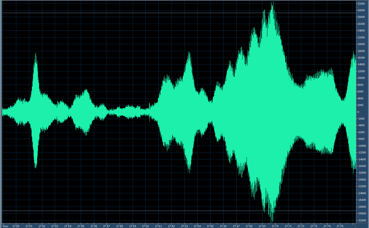
Figures 4 and 5, below, depict the rapid amplitude variations using a transmitted 4 kHz tone as an amplitude reference over a "Free Space Optical" path of approximately 15 miles (24km).  The horizontal axis is time and the vertical axis is linear amplitude.

Note the difference in horizontal time scales between the depictions, below:

Figure 4:
Scintillation of the laser-transmitted audio (4 kHz tone).
The time span of this particular graph is just over 250 milliseconds (1/4 second)
Click on the image for a larger version.

Figure 5:
Scintillation on the LED-transmitted audio (4 kHz tone).
In contrast to the image in Figure 4, the time span of this amplitude representation is nearly 10 times
greater - that is, approximately 2 seconds.  The rate and amplitude of the scintillation-caused
fading are dramatically reduced.
Click on the image for a larger version.

Laser scintillation:

As can be seen from Figure 4 there is significant scintillation that occurs at a very rapid rate.  The reference of this image is, like the others, based on a full-scale 16 bit sample.  Analysis of the original audio file reveals several things:

• While the "primary" period of scintillation is approximately 10 milliseconds (100Hz) but there is evidence that there are harmonics of this rate to at least 2.5 milliseconds (400 Hz) - but the limited temporal resolution of the test tone makes it difficult to resolve these faster rates.
• Other strong scintillatory periods evident in the audio sample occur at approximate subharmonics of the "primary" scintillatory rate, such as 75 and 150 milliseconds.
• The rate-of-change of amplitude during the scintillation is quite rapid:  Amplitude changes of over 30 dB (a factor of 1000) can occur in just 20 milliseconds.
• The overall depth of scintillation was noted to be over 40dB (a factor of 10000) with frequent excursions to this lower amplitude.  It was noted that this depth measurement was noise-limited owing to the finite signal-noise ratio of the received signal.

LED scintillation:

Figure 5 shows a typical example of scintillation from the LED using the same size emitter aperture as the laser.  Analysis of the original audio file shows several things:

• The 10 millisecond "primary" scintillatory period observed in the Laser signal is pretty much nonexistent while the 20 millisecond subharmonic is just noticeable.
  
• 150 and 300 millisecond periods seems to be dominant, with strong evidence of other periods in the 500 and 1000 millisecond range.
• The rate-of-change of amplitude is far slower:  Changes of more than 10 dB (a factor of 10) did not usually occur over a shorter period than about 60 milliseconds.
• The overall depth of scintillation was noted to be about 25 dB (a factor of about 300) peak, but was more typically in the 15-18dB (a factor of 32-63) area.

One of the more interesting results of this experiment was how minimally the severe amplitude distortion experienced with the laser actually degraded the overall intelligibility of human speech.  While the tones and brief music clips were clearly badly distorted, it could be argued that with the segment including speech, the degree of that distortion was not as apparent.  Clearly the voice content was being badly "chopped up" by the severe amplitude fluctuations, but with the redundant nature of speech and the fact that the drop-outs were quite brief in comparison to the duration of speech elements (sounds, syllables) it is quite reasonable to be able to expect the brain to fill in the gaps and make sense of it all.

A "Scintillation Compensator":

Despite the redundant nature of the speech maintaining reasonable intelligibility, it became quite "fatiguing" to listen to audio distorted in this manner so another device was wielded as part of an experiment:  The "Scintillation Compensator", the block diagram being depicted in Figure 6, below.

Figure 6:
Block diagram of the "Scintillation Compensator" system.
Click on the image for a larger version.

This system is essentially a "Keyed AGC" system using a low-level 4 kHz tone from the transmitter as an amplitude reference for a tracking gain cell at the receiver:  If the amplitude of the 4 kHz tone being received from the distant transmitter goes down, the gain of the audio in the receiver is increased by the same amount and vice-versa.  The effect of this device is quite dramatic as the clip in Figure 7, below, demonstrates:

Figure 7:

Audio clip with a"Before" and "After" demonstration

of the "Scintillation Compensator" 
Music:  "Children" by Robert Miles, used
in accordance with U.S. Fair Use laws.

One of the more striking differences is that in the "before" portion, the background hum from city lights remained constant while in the "after" portion it varied tremendously, more clearly demonstrating the degree of the amplitude variation being experienced.  What is also interesting is that the latter portion of the clip is much "easier" (e.g. less fatiguing) to listen to:  Even though syllables are lost in the noise, being obliterated by hum rather than silence in the first part of the above clip, the fact that there is something present during those brief interruptions, even though it is hum, seems to appease the brain slightly and maintain "auditory continuity".

It should be pointed out that the "Scintillation Compensator" cannot possibly recover the portions of the signals that are too weak (e.g. lost in the thermal noise and/or interference from urban lighting) but only that it maintains the recovered signal at a constant amplitude.  In the first portion of the clip in Figure 7 it was the desired signal level that changed while in the second portion it was the background noise that changed.  In other words, in both examples given in Figure 7, the instantaneous signal-to-noise ratio was the same in each case.

Practical uses for all of this stuff:

The most important point of this exercise was to demonstrate that a larger aperture reduces scintillation - although that point might be a bit obscured in the above discussion.  What was arguably more dramatic - and also important - was that the noncoherent light source seemed to be less susceptible to the vagaries of atmospheric disturbance.  This observation bears out similar testing done over the past several decades by many others, including Bell Labs and the works of Dr. Olga Korotkova.

For a brief bibliography and a more in-depth explanation of these effects visit the page "Modulated Light DX" - LINK - particularly the portion near the end of that page.

The reduction of scintillation has interesting implications when it comes to the ability to convey high-speed digital information across large distances using free-space optical means under typical atmospheric conditions.  Clearly, one of the more important requirements is that the signal level be maintained such that it is possible to recover information:  Too low a signal, it will literally be "lost in the noise" and be unrecoverable.

As the demonstrations above indicate, the "average" level may be adequate to maintain some degree of communications, but the rapid and brief decreases in absolute amplitude would punch "holes" in data being conveyed, regardless of the means of generating or detecting the light.  Combating this would imply the liberal use of techniques such as Forward Error Correction (FEC) and interleaving of data over time - not to mention some interactive means by which "fills" for the re-sending of missing data could be automatically requested.  The "'analog' analog" to these techniques is the aforementioned ability of the human brain to "fill in" and infer the missing bits of information.

While lasers are well-known to be "modulatable" at high rates, doing so for LEDs is a bit more problematic due to the much larger device (die) sizes and commensurate increase in device capacitance.  To rapidly modulate an LED at an ever-higher frequency would also imply an increase of "dV/dT" (e.g. rate of voltage change over time) which, given the capacitance of a particular device would also imply higher instantaneous currents within it, effectively reducing the average current that could be safely applied to it.  What this means is that it is likely that specialized configurations would required (e.g. drivers with fast rise-times at high current; structurally-small, high current/optical density LEDs etc.) to permit direct modulation of very high (10's of megabits) data rates.

Using the aforementioned techniques has rather limited utility when the free-space optical links extend out to many 10's of miles/kilometers owing largely to the vagaries of the atmosphere and the practical limits of optical flux with respect to "link margin" (e.g. the need to use safe and sane amounts of optical power to achieve adequate signal to recover information - particularly as the rate of transmission is increased) but it may be useful for experimentation.

Additional information on (more or less) related topics:

• Throwing One's Voice 95 miles on a lightbeam - link  - Details of experiments with high-power LEDs over a 95 mile (152km) optical path
• Voice on a Laser Beam - link - General information about using PWM techniques for Laser diode (and LED) modulation
• Gate Current in a JFET - link - The development of a highly-sensitive optical receiver that utilizes JFET gate current.
• The "Modulatedlight.org" web pages - link - This collection of web pages offers a large resource for many things related to free-space optical communications, including experiments, equipment and links to other related sites.
• For more information about the "Scintillation Compensator" and the "Audible S-Meter" used to set up the optical links, look at the page "An Audio Interface Device for Speech Bandwidth Optical Communications" - link

[End]

This page stolen from "ka7oei.blogspot.com".

Throwing one's voice 95 miles on a lightbeam

For more information about long-distance optical communications, go to the modulatedlight.org web page  (link)

This past weekend (September 15-16, 2012) was the 2nd part of the annual ARRL 10 GHz and up contest and we decided to use one of the highest-available amateur bands - the one known in the FCC rules as "275 GHz and up."  Actually, this covers a lot of territory including submillimeter radio frequencies and far infrared wavelengths, but the part that we are more interested in is that for which most of us are equipped to detect directly - light.

We've done this before, managing to have spanned 107 miles (173 km) on several occasions and even 173 miles (278 km) (read about those efforts here - link) so we weren't going to break any of our own DX (distance) records, but it's fun to do this, anyway - and it gave us an excuse (as if we really needed one...) to go out and test some new gear that had not yet been tested over anything but relatively short (20 km or so) paths.

The two locations for the stations were about 96 miles (154 km) apart with Ron and Elaine Jones (K7RJ and N7BDZ) being at the far end at an elevation of about 5600 ft (1700 m) ASL near Park Valley, Utah in the extreme northwestern corner of Utah, a few miles from where the U.S. Transcontinental Railroad was joined for the first time in 1869 and only a few hundred meters away from the historic stagecoach route that paralleled part of that later railroad.  Along with friends Gordon (K7HFV) and Gary (AB1IP), I  was closer to home at about 9300 feet (2830 m) near a minor protuberance known as "Bountiful Peak" about 10 miles (16 km) north of Salt Lake City.  As it turns out, the path is a grazing one and were it not for the slight refraction of the Earth's atmosphere, it may not even quite be "line of sight."

We'd tried this same path during the first weekend of the 10 GHz and up contest but the thick veil of smoke from wild fires elsewhere in the western U.S. prevented a successful contact - although our light beam was occasionally just visible to the binocular-aided eye in Park Valley.  This time, however, the air was reasonably clear, only somewhat hazy from the still-burning fires:  Since we "almost" made contact a month ago we were confident that this time we would have no problems.

Figure 1:
The high-power red LED shining to the north-northwest.
The lights of Layton, Utah and surrounding communities
may be seen way below, in the background! The dot at the terminus
of the red shaft of light is the light from Ron's end of the path.
Click on the image for a larger version.

Soon after we arrived on site Ron shone a 500,000 candlepower halogen spotlight in our direction and immediately we noted a lone, flickering, yellow-red dot in the blackness "above" the last ribbon of visible lights from the populated areas of Layton and Ogden about a mile (1600 meters) in elevation below us.  Using this as a visual reference I swung my high-power LED in his direction, using the Rayleigh-scattered shaft of red light as a guide, and immediately Ron reported that it was easily the brightest light visible:  Considering that there were only a small handful of lights visible from his dark, rural location, anyway, this wasn't saying much, but if anyone where to have dropped by and looked in that direction they would have seen the bright, red light and asked, unprompted, "What's that?!?"

Using our light as a guide Ron immediately fine-tuned his pointing and soon, a very obvious red light appeared in the darkness.  Initially starting out with the lower power 3-watt LED he soon switched to the much higher-powered 20-30-ish watt LED and the red dot in the distance was even more striking than before.  The dot at the end of the red shaft of light in the above picture was from Ron's LED.

Soon after we brought our transmitters up to full power we reduced them again to 1/4-1/15th as each other's signals were strong enough that there was noticeable distortion in the received audio - and it also allowed us to run full-duplex (e.g. both sides being able to send and receive simultaneously) without intercepting as much of our own, scattered transmit light and causing acoustic feedback between our speaker and microphone.

This was the first actual "long distance" test of the Phlatlight-based optical transmitter - these using CBT-54 LEDs and permitting a 20dB improvement on the audio received at the far end.  This also was the first test of some APD (Avalanche PhotoDiode) based optical receivers that I'd built some time ago (see the link at the bottom of the page) so we set about reduce each other's LED currents to do a sort of "limbo" dance - that's to say we wanted to answer the question "How low can we go?"

It immediately became apparent that even though we could read the Phlatlight modulators' current with a resolution of 0.1 amp, this was still too coarse when we got down to the lowest readable current and were still able to hear each other, so Ron switched to the older 3 watt Luxeon on which the LED current could be measured and adjusted down to the single digits of milliamps.  As it turned out, speech was copyable - with some difficulty - down to the 40-50 milliamp range with the old receivers but the APD receivers extended this down to around 20 milliamps - an approximately 6-10dB improvement, a number that agreed reasonably well with what had been calculated using similar measurements done at home on my "Photon Range" using a very dim LED and test receivers.

Practically speaking this meant that at full power with the Phlatlight LEDs we had about 50dB of  excess signal at the output of the receivers as compared to the minimum possible signal level using baseband speech and the "naked" ear.  Switching to MCW (tone-modulated Morse code) we could extend this by another 6-10dB and the the use of narrowband digital signalling techniques (such as WSPR or QRSS CW - very slow Morse) could have extended this by even another 20 dB or so.  The implication of this is that, in theory, we could communicate over that distance with only a milliamp or two of LED current!

Figure 2:
This time, a high-power green LED!
Click on the image for a larger version.

Satisfied with our tests I switched to a green CBT-54.  Interestingly - but not too surprisingly - Ron reported that subjectively the green LED wasn't really any brighter than the red had been.  On previous tests at much shorter distances (a few 10's of miles/km) the green far outshone the red owing to the fact that the human eye is at least 5 times as sensitive to green than the wavelength of red LED that we were using.  For these distances the atmospheric attenuation was sapping the vast majority of our light since the shorter (green) wavelengths are attenuated at a far higher rate than the longer ones, a fact that explains red sunsets and that we observed, at the beginning of our testing, that his white, halogen spotlight appeared to us as distinctly yellow/red in color.

The silicon photodetector didn't fare any better since it had far less sensitivity at green than red, the two factors (atmospheric and the Si sensitivity) adding up to between 20 and 30dB in degradation - assuming that the subjective measurement of "equal" brightness between red and green was correct.  As it turns out the degradation was probably far greater than that as the APD-based receiver could hardly detect voice at all, but this may have been also due, in part, to the fact that the gain of a standard APD drops off precipitously with shorter wavelengths and that it was likely not focused properly for green light due to chromatic aberration of the Fresnel lens!  In retrospect we should have switched to a receiver with a larger, "non-APD" detector - and thus less sensitive to misfocusing due to chromatic aberration.

In addition to using high-power LEDs, we also exchanged 2-way communications using plain, ordinary, cheap low-power red LED laser pointers.  The signals were far weaker - mostly owing to the lower optical power of the laser pointer - but each other's lasers were visible to the naked eye over the distance.  Because of the combination of the laser's (relatively) coherent light and its small exit aperture (small beam diameter) the scintillation (fading) on the laser-based link was terrible while on the LED-based link it was only just noticeable.  Some of the methods and techniques to communicate using laser pointers may be found in the September 5th entry of this blog.

After several hours of standing around in the dark on the mountain, we decided that it was getting early (approaching 2 AM!) and packed things up and made our way down the mountain.

Overall, it was a fun little jaunt giving us a healthy dose of nerdiness... enough to last for a few weeks, anyway!

Afterward:

While we run these tests, we'll often play something from portable audio players so that we have a continuous source of sound.  In this case, one of the audio sources that I used was from a Soldersmoke podcast.

For the heck of it, I emailed Bill, N2CQR, who produces this podcast and he put it on his blog page (link) as well as commenting on it in his next Soldersmoke podcast (link)!  This may have had something to do with this post appearing on Hack-A-Day (link)!

Links from the "Modulated Light" (link) web site:

• Using Laser Pointers for voice communications -  This page describes in more detail the methods by which one may successfully use inexpensive laser pointers to cast voice through many miles of the ether!
• A Highly-Sensitive Optical Receiver Optimized for Speech Bandwidth - This is one of the most sensitive speech-range optical receivers yet devised that uses standard photodiodes and is much more sensitive than the simple receiver depicted in figure 1, above.
• Receiver for low-bandwidth optical (through the air) communications using an Avalanche Photo Diode (APD) - This optical receiver is an enhancement of the one above, achieving another 6-10dB of ultimate sensitivity using an APD.  This receiver is about as sensitive as you can get without resorting to an exotic red-sensitive photomultiplier tube!
• A "Cheap" Optical Transceiver lens assembly - If you really want to improve your receive sensitivity, the best way to do this is with a large lens.  This article describes how one could use inexpensive foam-core poster board to make an assembly that will focus the distant light on the detector diode of an optical receiver.
• A "Mini" full-featured Pulse Width Modulator for high-power LEDs and laser diodes -This describes a simple, computer-based PWM modulator that will not only transmit audio, but generate test tones as well.

Be sure to check out the "ModulatedLight.org" web site's other pages as well!

[End]

This page stolen from ka7oei.blogspot.com