The Comcraft CTR-144 FM transceiver - A "multi-mode" solid state 2 Meter transceiver from the early 1970s.

Comcraft
Logo

Back in 1972 an ad appeared in the Ham magazines for something that probably seemed amazing at the time:  A solid state transceiver that covered the entire 2 meter amateur band (144-148 MHz - plus adjacent MARS and CAP frequencies) and did not need crystals!  This was the Comcraft CTR-144.  This radio cost $389.95 according to an advertisement in the January, 1972 issue of 73 magazine and was later listed at $489.95 in an ad in a 1973 73 Magazine advertisement (see Figure 6):  These prices are equivalent to over $3000 in 2026 dollars - for a two meter transceiver!

About Comcraft

Figure 1:
The Comcraft CTR-144 - a VFO solid-state 2 meter
FM/AM transceiver from the early 1970s.  A ham today
would probably be at loss when trying to use it!
The large knob is for tuning the receiver while the "VFO
Tuning" is for the transmitter frequency.  Aside from the
"tune" and "load" controls the rest are self-explanatory.
Click on the image for a larger version.

I haven't been able to find much about the Comcraft Company, other than it was in Goleta, California and that it seemed to exist from at at least 1971 until some time after 1976 when they released one of the earliest synthesized 2 meter transceivers, the CST-50.  I suspect that they may have made products for other markets, but I haven't been able find additional information.

More about the CTR-144

The CTR-144 is a "multi-mode" 2 meter transceiver in the sense that it can operate using both FM and AM - the latter being still present on the band in the early 1970s, but on its way out of common usage.  Compared to radios made since, this is an "odd duck" in the sense that it has separate tuning for the receiver and transmitter, both using VFOs - although it can accommodate three internal and one front-panel crystal for transmit for frequently-used repeaters and those applications that required good frequency stability and accuracy (e.g. MARS, CAP).  In other words, it doesn't have a conventional switch for a +/- 600 kHz repeater offset like that of modern radios, but rather you have to tune the transmitter and receiver separately to the repeater's input and output frequencies, respectively.  Additionally, it has a built-in power supply which allows it to operate from 120 Volts AC as well as a 12 volt input and provisions for an internal battery pack for "portable" use.

Figure 2:
The power amplifier section of the CTR-144 - solid-state
from the early 70s.  The "tune" and "load" air-variable
capacitors are visible, as is the side-mounted antenna jack.
Click on the image for a larger version.

As with some other radios recently featured on this blog, I acquired this one from a silent key friend of mine - and even into the early 2020s, he'd occasionally use this transceiver on some of the local repeaters that didn't require a subaudible tone.  It also has a very wide range "S-meter" which, unlike meters on most modern FM transceivers, would give a repeatable, reliable indication of signal strength over a range of just a microvolt or so to extremely strong. ¹  Being able to operate from a 12 volt vehicle and combined with the S-meter's wide dynamic range also  made it a decent receiver for direction-finding not only with a small directional antenna, but to know when one was getting very close to the transmitter itself.

About the transmitter

The transmitter isn't particularly high-power:  The specifications state that it's finals are rated for 12 watts input power with about 6 watts out. ² Considering the efficiency of early 1970s VHF power transistors, the output power of this transceiver is still in the range of 4-6 watts across the band, depending on frequency and supply voltage - plenty of power for local and moderate-distance repeaters when used with a modest outdoor antenna.

Figure 3:
Before the mid-late 70s there were no specific FCC rules
for the spectral purity of VHF transmitters, but current rules
still allow transmitters of that vintage to be used despite this.
Were it made today, the CTR-144 would not pass muster.
Click on the image for a larger version.

Out of curiosity I checked this transceiver's spectral purity on my service monitor (see Figure 3) and I wasn't terribly surprised at what I found:  While there were a few minor non-harmonic spurious emissions that were at least 40dB down from the carrier, the second harmonic was around -27 dBc - roughly 4 milliwatts.  While this would not be given a "pass" if the radio was made today (the current rules state that spurious/harmonic signals of a transmitter with 25 watts or less should be -40 dBc) there were no such rules prior to about 1977.  As noted in the current FCC rules, (§ 97.307(e)) a radio from this era is exempt from these rules but, if using a radio such as this causes interference, the onus is still on the amateur to resolve any issues.

If one looks at Figure 1 you'll see that there are two tuning knobs:  The larger one - which is coupled to the slide rule that covers 144-148 MHz - is for the receiver, but the smaller one, labeled "VFO Tuning" is what sets the frequency of the transmitter and it is completely independent of the receive frequency.  What this means is that if you wish to use a repeater, the receiver is tuned to its output and the transmitter is set to its input frequency which, in the day, may have been a bit of a challenge:  The VFO Tuning (for transmit) knob doesn't have a great deal of tuning resolution on its dial so getting it "on frequency" back in the day probably meant setting the knob as close as possible visually and then getting "talked in" to the proper frequency.  When using this transceiver, my friend would have a frequency counter handy to allow him to dial in the transmit frequency precisely and monitor it for drift.

The transmit VFO itself operates from 7 to 9 MHz and this frequency is then mixed with a 65 MHz crystal to yield 72-74 MHz - and this is then doubled to the 144-148 MHz 2 Meter band.  With this scheme the transmit frequency could be reasonably stable as the most drift-prone component, the 6-9 MHz VFO, was operating at a low frequency.

A close inspection of  the front panel  in Figure 1 will reveal - along the right edge of the front panel - both a "Tune" and "Load" control.  For anyone using a radio with vacuum tube finals, controls labeled thusly would be familiar, but as this transceiver has a solid state amplifier these simply provide peaking/matching for final amplifier as indicated on the "S" meter rather than the "dip and load" of the older technology.

Figure 4:
The bottom of the CTR-144 showing the
rather hefty power transformer and, on top,
the doubler stage for the transmit chain.
The modulation transformer can be seen to
the left of the large, blue capacitor.
Click on the image for a larger version.

To produce frequency modulation it is the 7-9 MHz VFO itself that is modulated, but if a crystal is used, phase ³ modulation is applied to its oscillator's output prior to being multiplied by 18 to the desired transmit frequency.  For AM, high-level modulation is accomplished by using an audio amplifier to modulate the +12 volt supply for both the final amplifier transistor and its driver via the windings of an autotransformer - a rather "old school" way of doing it, but one that eliminates the need for another, higher-voltage power supply to achieve the desired peak output power. ⁴

About the receiver

While schemes to up-convert a low-frequency VFO for transmitting had been used for a long time, the way this transceiver goes about receiving is a bit more interesting and complex.  While more modern analog receivers would generate a local oscillator near the receive frequency and convert the desired signal to one or more lower-frequency IF (Intermediate Frequency) stages where a single channel would get demodulated, this works more like the receive section of a transverter in that the entire 2 meter band is is down-converted to the range of 14-18 MHz using "high-side" injection (e.g. the local oscillator is above the receive frequency) at 130 MHz from the same 65 MHz crystal as is used for transmit.

The receive VFO - the one tuned by the large knob with the frequency indicated by the slide rule - tunes across the 14-18 MHz IF to down-convert the received signal down to a fixed IF of 2 MHz where it is filtered and demodulated by a CA3075 integrated circuit.  The receiver front end itself uses some MOSFETs for amplification and mixing - a technique still used on superheterodyne receivers made today - and its sensitivity is as good as any receiver made today.

Using the CTR-144 on the air today

Figure 5:
The front end and receive section of the CTR-144.
The three-section air-variable capacitor tunes the local
that down-converts from the 14-18 MHz first IF to the 2 MHz
second IF where an integrated circuit is used for audio
demodulation.  In the upper-left is the MOSFET front-end
and filtering that give this radio good sensitivity - even by
today's standards.
Click on the image for a larger version.

Using the CTR-144 today is admittedly awkward compared to a modern radio, provided that the lack of subaudible tone for transmit won't be an issue.  The receiver's slide-rule dial will get you "pretty close" to frequency, but unless the signal is actually present, you won't be able to tune it in for certain.  For simplex use, once you have tuned the receiver, there is a "Spot" switch that will inject a weak signal into the receiver that you can use to tune the transmit VFO to the same frequency by listening for and zero-beating it:  In this way the transmit and receive frequencies will be very close to each other.

Repeater operation is another matter. ⁵  Back in the 1970s you might have spent a few dollars to get transmit crystals for your favorite repeaters which would circumvent the problem of not knowing one's exact transmit frequency with the VFO.  But what if you didn't have a transmit crystal for the frequency?  Here, the "Spot" button is less-useful since, unless you happen to tune in someone's signal as they are transmitting to the repeater on its input frequency, there would normally be no signal at all to which you could precisely set its frequency.  While my friend, in later years, had a frequency counter in his ham shack so that he could determine precisely the transmit frequency, this luxury that would have been unthinkable when this radio was first introduced. ⁶

Figure 6:
A Comcraft advertisement from
the April, 1973 issue of
73 Magazine
Click on it for a larger version.

Final comments

• When I first placed this transceiver on my workbench, it worked perfectly (although I haven't tried the built-in AC power supply) aside from two of the #47 dial lamps having burnt out.
• When the sensitivity was checked, it was only slightly deaf, but just a couple of minutes of time with the service monitor and tweaking the RF and IF stages brought it into specs.  It's interesting that while the manual (see link, below) has some "adjustment" information, it doesn't have a fully-detailed alignment procedure for the transceiver, likely because, as is true today, few people would have access to the necessary equipment to accomplish the task.  As it was the manual and schematic informed me as to how it worked I was able to come up with a procedure "on the fly" to bring the radio back up to snuff.
  
•  When 2 Meter FM first appeared, it had not yet standardized on what we now call "Wide" FM (e.g. +/-5 kHz deviation).  Different channel spacings and modulation widths could be found in different parts of the country, including +/- 15 kHz deviation - particularly on UHF.  The manual for the CTR-144 specifies a deviation of +/-7.5 kHz - yet another "standard"!
• The specified receiver bandwidth is 22 kHz which is somewhat wider than the typical 15-17 kHz for a "wide" FM receiver intended for +/-5 kHz deviation.  With this bandwidth - plus the probability of the receiver's VHF frequency not being centered - an adjacent-channel repeater (15 or 20 kHz away, depending on the spacing in your area) is likely to result in received interference.

Comcraft CTR-144 manual

I was fortunate enough to find the manual for this transceiver in my friend's files which has been scanned and may be found at this link:  Comcraft CTR-144 Manual (35 MB, .PDF).  At the time that this blog was posted, this manual was not to be found anywhere else on the Internet.

* * * * *

Footnotes:

1. On most FM transceivers, the S-meter will start indicating on very weak (and possibly noisy) signals and hit the "peg" (e.g. full-scale) even on a signal that is only modestly strong.  What this means is that for direction-finding purposes, most modern FM transceivers will give a "pegged" S-meter indicating even if you are some distance from the transmitter.  The CTR-144 on the other hand reaches full scale only if you happened to be right next to the transmitter while at the same time it starts indicating on a signal that is almost too weak to copy meaning that it could be used both at a great distance or in the final search for an unknown transmitter. 
2. Until the mid-late 1970s, amateur radio power limits were specified as input power to the final amplifier stage.  This method of transmitter power was likely an artifact of the days before RF power meters were common:  It's trivial to calculate the input power to the final amplifier if one knows the current and voltage, but that isn't the case for trying to measure RF power.
3. "Phase" modulation doesn't change the frequency directly but rather it "wiggles" the phase of the signal in accordance to the applied audio whereas actual "Frequency" modulation does change the frequency of the signal - in this case, by electrically shifting the VFO frequency:  Mathematically, the two are related since, if you could continually change the phase, frequency modulation would be the result.  With "FM" as used in the amateur service, one need only be able to modulate down to 200 Hz or so for voice meaning that with phase modulation, you could "temporarily" change the phase enough to effect a temporary de-facto frequency shift.  As the amount of change from a single phase modulator stage is quite small (perhaps +/- 60 degrees) this is usually applied at a lower frequency - in this case, at the 8 MHz crystal frequency and since this is multiplied by a factor of eighteen, our original +/-60 degrees of phase change becomes (18 * 60) 1080 degrees which is enough to appear as an adequately-modulated "FM" signal.  Mathematically, if one boosts the "highs" of the audio at a rate of 6dB per octave (e.g. doubling the deviation with every doubling of frequency) a signal generated using "FM" is indistinguishable from one that was originally phase modulated.  In fact, it is "PM" (Phase Modulation) that we use on "FM" as amateurs:  The "highs" in the audio are boosted (e.g. "emphasized") on transmit as they are the first to get noisy with a weak signal, and on receive they are restored back to their original level (e.g. "de-emphasized") which effectively reduces the amount of noise that is heard and makes weak, noisy signals more "listenable".
   
4. "High-level" modulation typically refers to applying the audio to the output RF stages(s) of a transmitter by increasing/decreasing the supply voltage.  Traditionally, this was done with an audio amplifier driving modulation transformer:  On peaks with 100% modulation the voltage applied to the final amplifier is approximately doubled, yielding the  four times the peak envelope power - but it also allowed the voltage to go to near zero at the other extreme.  On this transceiver, an audio amplifier drives an auto transformer (e.g. one with a single, tapped winding).  With no modulation, the 12 volt power supply for the finals goes through it unchanged, but with audio, the transformer action allows the requisite 24-volt(ish) peaks to be applied to the amplifier stage - all without needing the complexity of a 24 volt power source.  This method was "old" even when this radio was made, but it is simple and effective.
5. When this transceiver was made it was fairly rare for an amateur repeater to use a subaudible tone as doing so would mean that an amateur using it would not only have to have the proper crystals (for most radios of the day) but also a means to produce the needed subaudible tone frequency,  Later, in some areas subaudible tones were introduced when a geographically-adjacent repeater was on the same frequency to prevent users in an overlap area from bringing up both repeaters.  In some cases in amateur radio service, subaudible tones are used owing to occasional interference issues:  This is often considered to be a "band-aid" solution to a problem that is often due to the repeater's receive signal path not being able to adequately reject off-frequency signals (e.g. overload) - but sometimes it might be needed on a "busy" site where other users' gear isn't as well-filtered as it should be.
6. Back in the early 1970s a frequency counter of any sort would be a somewhat rare and expensive piece of test equipment - and this would be particularly true for one that could operate at VHF!  By the late 1970s and early 1980s technology had progressed to the point where such devices were more affordable and available to the average amateur. 

 * * * * *

This page stolen from ka7oei.blogspot.com 

 

[END] 

The Morrow CM-1 receiver - A relic of the cold war's effect on amateur radio

Figure 1:
The front panel of the Morrow CM-1 CONELRAD monitor.
The meter indicates relative signal strength and below it is the
on/off/volume control.  The dial - with a pair of "CD"
markings, is a smooth-tuning reduction drive - which is also
very accurate.  Shown here, it's on and tuned to a local station.
Click on the image for a larger version.

If you were an amateur (Ham) radio operator in the late 1950s and early 1960s, you  had a broadcast radio turned on in the background whenever you were on the air - or at least you should have!

The reason for this was spelled out in the FCC rules:  Beginning January 1, 1957, Section 12.192 required all amateur radio stations to monitor a broadcast station - at a minimum of ten minute intervals - to see if it transmitting, while they (the amateur) was on the air.  If the station had gone off the air, it was then required that the amateur determine if this was because of a CONELRAD alert - and if so, immediately cease transmitting.

What was CONELRAD?

CONELRAD, short for "CONtrol of ELectromagnetic RADiation", was a system - part of the U.S. Civil Defense - where, if an imminent attack of Soviet bombers was detected, ALL radio stations - commercial (AM , FM and TV) and amateur - were to go off the air to prevent their signals from being used as directional signals for navigation by the enemy.  The exception to this was that some of the AM broadcast stations were to ultimately occupy either 640 or 1240 kHz - but only for a few minutes at a time, the frequencies to be used by several different stations during that period - in a "round-robin" sort of system.  The "musical chairs" of transmitters, frequencies and locations was intended to make it difficult for the Soviet bomber to use them for navigation.

If you have seen an AM broadcast receiver intended for the U.S. market from the time period when the CONELRAD system was in existence (from about 1951 to 1963) you may have noted that at 640 and 1240 kHz there are triangular marks - often with the letters "CD" in them (the Civil Defense logo) - on the dial signifying the two CONELRAD frequencies - and these symbols are clearly visible on the tuning dial in Figure 1.  The intent of this is that civilians would tune to those frequencies to receive civil defense instructions during the "on" periods of the broadcast station near them.

Figure 2:
Rear of the CM-1.  The terminals connect to normally-open
contacts of the relay (if fitted) and the wire antenna can be
seen emerging from the chassis.  Between the two is a
potentiometer for adjusting the S-meter and relay sensitivity.
Click on the image for a larger version.

How it worked

As you might imagine, this system was cumbersome.  All stations had to be alerted in some way and "key" stations - perhaps notified via a wire service - would turn their transmitters off-on-off and on again in five second intervals and then transmit a 1 kHz tone for 15 seconds:  As transmitters of the day weren't designed to be "short-cycled" in this way, it was hard on the equipment - sometimes leading to failures.  There was also the requirement that some transmitters - and their antenna systems - change from their normal frequency to either the 640 kHz or 1240 kHz CONELRAD channel - a further complication - to participate in the on/off "round robin".

Needless to say, this system had several well-publicized false alarms as well as failures when tested over the years that it was extant.  Eventually, because of the implementation of ballistic missiles rather than piloted bombers, its reason for existing ceased in 1963.

How it affected amateur radio operators

As noted earlier, if you were an amateur radio operator, you were required to monitor a local broadcast station, while you were on the air, at least every ten minutes:  If the radio station went off the air, the idea was that you were to check for a CONELRAD alert and if it was happening, immediately stop transmitting.

Figure 3:
Top of CM-1 chassis as seen from its left side.  In the fore-
ground is the tuning capacitor, IF transformers and amplifier
tube and main filter capacitor.  The 6C4, if installed, would
be plugged in the empty socket just visible behind the tuning
capacitor.  It's well laid-out - even the audio transformer is at
an angle to minimize coupling to the AC power transformer.
The antenna wire is lightly coupled to the preselector circuit.
Click on the image for a larger version.

It's difficult to know these days how well the average amateur radio operator adhered to this rule, and for those that did, doing so certainly added a bit of complexity and awkwardness to their operating style.  A number of article appeared in the amateur radio magazines at the time describing how to "automate" the detection of the local radio station going off the air - typically by monitoring the AGC voltage of an inexpensive radio and sounding a buzzer or turning on a light.

There were also some receivers designed for just this purpose.

The Morrow Radio Mfg. CM-1

The Morrow CM-1 was one such receiver.  The receiver pictured was found among the effects of a good friend - and fellow amateur radio operator - that passed away several years ago, sitting dusty on a shelf in his basement.  After careful inspection, I was surprised to see that it had no bad capacitors:  The components used in its construction - particularly the capacitors - are all good-quality Cornell Dubilier (all are ceramic disk types other than the main filter) - and they seemed to be a cut above those found in a typical, cheap domestic radio of the time and it worked perfectly the first time it was turned on - and I haven't even bothered checking the tubes!  Even the main electrolytic filter capacitors are still in excellent shape - likely a result of the receiver having spent the past six-plus decades in a cool, dry basement.

Figure 4:
Schematic of the Morrow CM-1.  Despite the somewhat unusual tube line-up, it functions
the same as a typical "All American Five" superheterodyne receiver of the era, complete
with a 455 kHz IF.  The main difference is that it has provisions for connecting to an external
alarm or light based on the presence/absence of a signal using the (optional) 6C4 tube and the relay.
Click on the image for a larger version.

A "brief" circuit description  (Refer to Figure 4)   While many "AA5" receivers use a resonant loop - either a ferrite stick or a coil wound on the back panel of the chassis for an antenna - the CM-1 uses just a short piece of wire, depicted in the upper-left corner of the diagram connected to C1, one half of the tuning capacitor and inductor "L1".  This and the 50-100pF series capacitor "lightly" couple a short piece of wire to the resonant circuit.  This works, but its effects can be swamped if a long piece of wire (more than a few feet/meters) is used which can spoil image rejection an cause the radio to overload on strong signals. The 6EA6 converter doubles as both the local oscillator - its frequency determined by the other half of the tuning capacitor C2 and L2 - and mixer as it converts and amplifies the received signal to the Intermediate Frequency (IF) of 455 kHz via its plate through transformer T1 which forms a selective band-pass filter.  Following T1 is a 6BJ6 which functions as an amplifier at 455 kHz and this goes to T2, another 455 kHz IF transformer, and then to the 6AV6 diode/detector/amplifier tube.   The secondary output of transformer T2 applies the 455 kHz signal to a diode section and since its cathode is grounded, it causes that part of the transformer to go negative with the rectified DC voltage as well as the detected audio:  The received audio is then coupled via a 0.01uF capacitor and 10 MegOhm potentiometer to the triode section of this tube for amplification where the audio is then coupled to the plate of the 6AS5 - its grid biased slightly negative by the 220 Ohm resistor in the cathode - and amplified.  Functioning as a "Class A" single-ended audio amplifier, transformer T3 couples its high-impedance plate to the low-impedance speaker. Referring back to the bottom of the secondary of T2 where the audio is tapped, the negative DC voltage that is also produced there is in proportion to the amount of signal getting to the 6AV6 detector tube and ultimately, the strength of the signal to which the radio is tuned.  This voltage is smoothed to remove the 455 kHz IF by a 250pF capacitor and then sent to one of the grids of the 6EA6 converter tube through the antenna-tuning inductor, L1 and also to one of the grids of the 6JB6 IF amplifier via the secondary of T1 and when the voltage gets more negative, its sensitivity is reduced.  In this way the "AVC" (Automatic Volume Control) is formed so that both weak and strong stations produce similar amounts of audio. This same AVC voltage is also sent to the (optional) 6C4 tube:  If this voltage is very negative - as it would be with a moderately strong signal - this tube is "cut off", but if the signal disappears and the AVC voltage is less negative, it will conduct and thus turn on the (optional) relay. For the signal level meter, a voltage divider using a 15k resistor  and 2k potentiometer (seen at the bottom of T1) sets the voltage threshold on one side of the 1 mA meter - the other side of which is connected to the cathode of the 6JB6 IF amplifier tube along with a 1k resistor to ground.  There are two mechanisms of action here for driving the meter:  If there is more signal into this tube, it conducts more current and the voltage goes up across the 1k resistor, but a higher signal will also result in a more negative AVC voltage which will negatively bias the tube and reduce the current.  It's this latter aspect that prevails:  A more-negative AVC will reduce the tube's conduction and also the voltage across the 1k resistor and when this voltage is lower than that across the 15k-2k voltage divider, the meter will move up-scale.   The final section is the power supply which consists of a transformer to isolate the circuit from the mains.  The high voltage is half-wave rectified by a "modern" (for the time) selenium diode and then filtered by one section of a two-part capacitor which is then decoupled by a 750 ohm resistor in series which then goes to another capacitor.  In this way, the voltage is reduced somewhat and better-filtered than it would be with just a single stage of smoothing.

The CM-1 is a compact, tube (valve) type superheterodyne receiver from this time period that was designed to indicate when a station went off the air.  As can be seen from the photo, it looks more like a piece of ham gear than the AM broadcast band receiver in that it has a "nicer" geared (and accurate) tuning dial and a meter than indicates the relative strength of the signal to which it is tuned.

Internally, he CM-1 itself is mostly an unremarkable receiver:  Electrically, it's a variant of the "All American Five" (AA5) superhet that was produced by the millions over about four decades, but with a few interesting differences.  Sporting a power transformer, all of the tubes use six volt filaments and with the isolation, it - unlike most later, cheaper versions of the "AA5" - it does not have a "hot" chassis (e.g. one that is connected to one side of the line cord) - but with a solid-state (selenium) rectifier rather than the typical 35W4 and a rather different six volt tube line-up than a typical AA5.  A 6BE6 as the converter, 6BJ6 as the IF amplifier, 6AV6 as the detector/amp and interestingly, a 6AS5 (a tube typically used in car radios) for the audio output.  As can just be seen in Figure 5, the 6AS5's "getter" shows discoloration and Figure 3 reveals that there is a slight stain around the audio transformer where some of its wax wicked onto the chassis due to heat, both indicating that this receiver has quite a few "on" hours!

An interesting departure from a typical AA5 is its antenna connection.  Most AA5s had either a ferrite loopstick or a large coil of wire wound on the cardboard/masonite/phenolic back cover of the receiver that doubled as an RF pre-selector, but this receiver simply has a piece of wire capactively coupled to the tuning network connected to one of the capacitor's gangs.

According to the manual, only 2-3 feet (50-95cm) of wire is necessary for reception and testing of this CM-1 indicated that this was true - but it also means that one must resist the temptation to connect it to a longer wire:  Doing so simply overloads the receiver and wrecks image rejection, particularly since the front-end preselector tuning is overcoupled to the antenna itself, effectively bypassing it altogether. 

I suspect that having a really sensitive receiver was not required in this application.  When monitoring for CONELRAD, one would probably use a local station with a strong signal:  Doing so would not only help with the fact that many AM broadcast stations had to reduce their power at night, but a weak/distant station would be interfered with with the onset of nightly skywave propagation which could, at times, cause signal levels to fluctuate wildly, resulting in false alarms.

During testing - with only the 2' (50cm) wire antenna - when placed outside, I found that the receiver was capable of picking up even the weaker signals across the broadcast band, but since it is a wire rather than a coil, it's non-directional and is far more prone to pick up local "E-field" noise energy than the typical "H-field" loop which is not only directional, but offers a degree of rejection of such noise.  Practically speaking, one could probably add a loop antenna, connecting to the wire and the grounded screw (one of the two used for the relay) on the back panel to improve reception in today's modern electrical environment.

Figure 5:
The other side of the top of the chassis.  In the foreground is
the power transformer and next to it is the 6AS5 audio amp.
The socket next to the 6AS5 is for the (optional) relay, driven
by the (also optional) 6C4.  The antenna tuning coil is visible
next to the tuning capacitor, almost against the front panel.
Click on the image for a larger version.

When I first removed the receiver from its chassis I thought that it was missing two tubes as evidenced by empty sockets, but I then realized that it had a selenium rectifier accounting for there being only four tubes and immediately wondered why there were two extra sockets.  A bit of "Google-Fu" found the manual online and I learned why:   This receiver could optionally be fitted with a relay in one of the sockets (this also required another tube - a 6C4 to detect the loss of signal and drive the relay) that was intended to operate a sounder, a light or some other means of indicating loss of signal.  I find it interesting that this relay and its driver tube were omitted as shipped from the manufacturer, but I suspect that this was a cost-saving measure - and it may have been enough for most amateur radio operators using this receiver to simply glance at the front-panel meter occasionally to see if a signal was still there.

Is it still useful?

The reason raison d'etre for this device ceased to be when, in 1963, the FCC rule requiring the amateur radio operator to monitor broadcast stations while operating was rescinded and removed from FCC Section 12.192, but since it's rather compact and has a speaker that dominates the top of the case means that it still works as a pretty nice AM broadcast receiver.  Whether or not one might think an AM-only receiver is still useful overall is another matter altogether!

Figure 6:
Bottom of chassis of the CM-1.  High-quality components -
including all Cornell Dubilier capacitors - are used
throughout.  The orange object left of center is the selenium
rectifier and the oscillator coil is just right of center.
Click on the image for a larger version.

The usefulness and practicality of this receiver is probably on par with most other vintage radios that one might collect and own:  They are not likely to be "everyday drivers" and more likely to sit on a shelf with other old radios - but this one, at least, has a particularly interesting bit of cold-war history behind its existence.

* * * * * * *

 This page stolen from ka7oei.blogspot.com

[END]

Revisiting the "Limited Attenuation High Pass" filter - again.

In several previous posts (See:  "A Limited Attenuation High Pass Filter" and "Revisiting the Limited Attenuation High Pass Filter" I described a "high pass" filter that offered low attenuation at high HF frequencies, but a controlled amount of attenuation at lower frequencies - this, to accommodate a fundamental fact about both HF propagation and direct-sampling Software Defined Radios (SDRs):  The two don't play nice with each other!

Note:

If you are using any direct-sampling Software Defined Radio to receive ALL of the HF spectrum simultaneously  - such as a KiwiSDR, Red Pitaya, RX-888, RX-666, TRX Duo to name but a few - you SHOULD read this page and understand why it is important to apply such filtering to maximize performance across HF.

In a typical receiver/antenna configuration, failure to reduce the lower HF frequencies with respect to the top of the HF spectrum (e.g. 10 meters) will result in comparatively poor performance.

As noted in the previous post(s), the problem is two-fold when it comes to broad-band SDRs that are intended to cover the entire HF spectrum all at once:

• HF noise power and signal level is (generally) inversely proportional to frequency.  At lower frequencies - say, 2-8 MHz - the noise power is far higher than it typically is at around 20-30 MHz.

• A direct-sampling SDR - or any receiver, for that matter - can tolerate only so much RF power on its front end.  Traditionally, this is a mitigated with the use of narrow-band RF band-pass filters, but this can't be done if one intends to be able to cover the amateur radio bands 160 through 10 meters (1.8-30 MHz).

With the aforementioned issues is yet another one:  Because the noise floor at 10 meters when it is "quiet" is so much lower than 80 meters (perhaps 40-50 dB during noisy nighttime conditions, 25 dB or so during quiet daytime conditions) there is an intrinsic disparity between the amount of sensitivity that is need to "hear everything" at the opposite ends of of the HF spectrum - but since a typical direct-sampling SDR is pretty much "flat", we end up with what might seem like a pair of intractible problems:

•  To accommodate the very strong signals and high noise levels at lower HF frequencies, the RF signal gain in front of the A/D converter must be carefully set to prevent overload.

• In order to "hear" the noise floor at 10 meters, the system gain must be set fairly high.

What these two factors, together, imply is that if we have enough gain to comfortably detect the noise floor at 10 meters, our receiver will be badly overloaded during strong-signal conditions on the lower bands.  Conversely, if we scale (e.g. attenuate) the input to accommodate the very large signal excursions, the receiver will simply be unable to detect signals at/near the "quiet" 10 meter noise floor.

Comments:

There will (hopefully) be the day that the upper HF propagation conditions improve greatly with the arrival of solar cycle 25 and at that time, strong signals will appear on the bands >=15 MHz.  When this happens, we will likely be faced with a problem similar to that which we are trying to solve here (e.g. very strong signals overloading the A/D converter).  At this time, the only recourse will likely be a means of using an external device to adjust the gain/attenuation in front of the receiver, probably using the existing I/O lines under receiver control.

Since the original posting of this blog entry I was made aware of an 1977 article on this very topic - you can read it HERE. (The article in question begins on page 3 of the PDF.)

A revised circuit:

Why talk about this issue a THIRD time?  I decided to make one that provided a better 50 ohm match across all frequencies than the previous versions.  This revised circuit may be seen in the figure below:

Figure 1:
Generic pre-emphasis network set for about 50 ohms.
Click on the image for a slightly larger version.

Some readers will recognize the topology of the circuit in Figure 1 as the classic pre-emphasis network found in the signal  path of FM video transmitters.  Whereas those circuits are typically designed for 75 ohms, this one is intended for a 50 ohm system - but careful observers will notice that 47 ohm resistors are used, instead:  For receive-only purposes, I have chosen the components in this article to be standard values at the expense of a slight increase in mismatch - but the VSWR of these circuits, when terminated at 50 ohms - is likely to be no more than about 1.1:1.

This circuit - compared with the previous versions - has the advantage that it presents a consistent source and load impedance across the frequency range, making it a bit more "friendly" in systems that may be impedance sensitive (e.g. following a band-pass filter, long coaxial cable runs, following/preceding conditionally-stable RF amplifiers.)  The obvious trade-off is that as compared to the previous version (which was based on a high-pass filter and some resistive bypassing) this circuit has definite limitations on how sharp and deep the "knee" may be at any given frequency as only a single inductor and capacitor are used.

By tweaking the values of R1, R4, C1 and L1 we can adjust both the amount of low-frequency attenuation and the frequency of the "knee" where the attenuation takes place - but for our purposes, we will be placing the center of that "knee" around 10 MHz to provide both the minimal loss at 30 MHz and adequate attenuation at and below 7 MHz.

Here are a few examples of values of R1, R4, C1 and L1 using standard-value components and approximate attenuation values at various frequencies:

R1 = 68 ohms  R4 = 39 ohms C1 = 390pF  L1 = 1uH DC attenuation:  7.3dB @ 2 MHz: 7.0dB  @4 MHz: 6dB @ 7 MHz: 4.6dB  @10 MHz: 3.4dB @ 14 MHz: 2.3dB  @28 MHz: 0.8dB	R1 = 120 ohms  R4 = 20 ohms C1 = 330pF  L1 = 0.82uH DC attenuation:  10.8dB @ 2 MHz: 9.8dB  @4 MHz: 8.1dB @ 7 MHz: 5.6dB  @10 MHz: 3.9dB @ 14 MHz: 2.5dB  @28 MHz: 0.8dB
R1 = 120 ohms  R4 = 20 ohms C1 = 270pF  L1 = 0.68uH DC attenuation:  10.8dB @ 2 MHz: 10.1dB  @4 MHz: 8.7dB @ 7 MHz: 6.5dB  @10 MHz: 4.8dB @ 14 MHz: 3.3dB  @28 MHz: 1.2dB	R1 = 100 ohms  R4 = 27 ohms C1 = 270pF  L1 = 0.68uH DC attenuation:  9.4dB @ 2 MHz: 8.9dB  @4 MHz: 8dB @ 7 MHz: 6.3dB  @10 MHz: 4.8dB @ 14 MHz: 3.6dB  @28 MHz:1.3dB

Figure 2:
Table showing some possible values for the circuit of Figure 1 and the example attenuation values.

 

In practice, several of these sections will likely need to be cascaded to achieve the desired amount of attenuation at the lower HF frequencies which brings up the question:  Could you not choose components to do this for a single section?  The answer is theoretically, yes - but the fact is that practical inductors - particularly the molded type - are quite lossy, departing from the intended attenuation curve, and achieving the predicted, higher amount of lower-frequency attenuation with a single stage can become problematic - so it's probably better to cascade several of these networks together, instead.

A practical example:

Figure 3:
The exterior of the four channel filter network.
Click on the image for a larger version

A practical example of such a network is one that is to be currently installed in the KFS (Half Moon Bay, CA) KiwiSDR/WSPRDaemon system.  There, four wideband antennas are available to feed the KiwiSDRs on site, so a box was constructed with four, identical pre-emphasis networks, each to feed its own receiver stack.

As is the case at the Northern Utah WebSDR, noise and signals at the lower end of the HF spectrum is often very much stronger than at the high end:  If amplification is added to allow the detection of the noise floor at 10 meters, there is the very high probability that the receiver will badly overload on HF signals from the lower end of the spectrum.

Each "channel" of the device depicted in Figure 3 is identical, consisting of two cascaded sections.  The first section is that from the upper-left quadrant of the table (R1=68 ohms, C1 = 390 pf) and the upper-right quadrant (R1=120 ohms, C1 = 330pF).  Rather than the use of molded chokes, the individual inductors were wound using 30 AWG wire on T25-2 toroids:  17 and 15 turns for the 1 uH and 0.82 uH inductors, respectively.

Figure 4:
The interior of the four-channel network.
The circuit is simple enough to be wired "Manhattan"
style on glass-epoxy PC board material between the
two center pins of the BNC connectors.
Click on the image for a larger version

As can be seen in Figure 4, the construction is very simple, requiring no circuit board at all when using standard, through-hole components.  The circuit was built into a die-cast aluminum box with the BNC connectors holding the piece of PCB material in place.

To secure the components - particularly the small, toroidal inductors - RTV sealant (white) was used to hold components in place and to prevent adjacent wires of C1/R1 and R2/R3 from coming into contact with each other.

This method of construction is very simple and effective, offering good performance into the VHF range when reasonable care is taken.  With the 20mm high dividers between the sections installed as shown, the channel-to-channel isolation exceeded 85dB (the limit of convenient measurement) at 30 MHz.

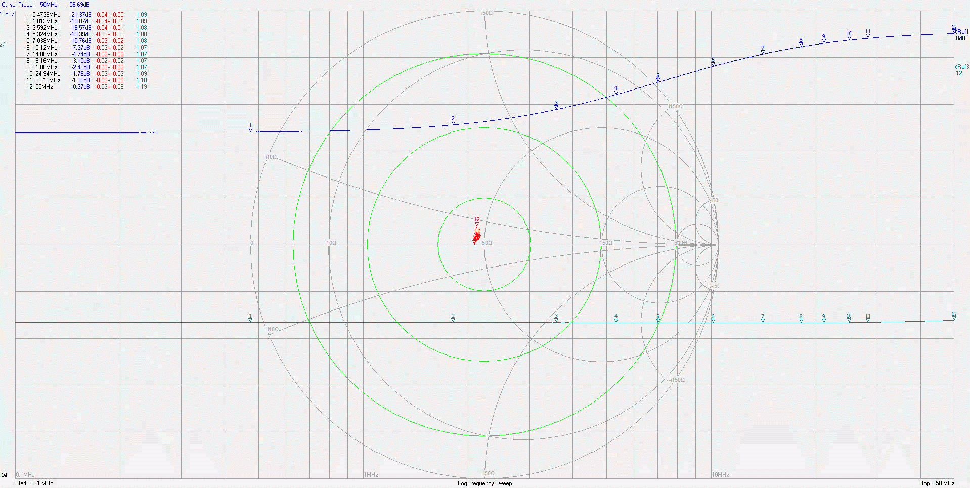
Figure 5, below, shows the typical response of the sections:

Figure 5:
The response of one of the sections as measured on a DG8SAQ VNA.
Click on the image for a larger version.

Because it can be a bit difficult to read, the values of attenuation and VSWR in the upper-left corner are reproduced below:

Frequency (MHz)	Insertion Loss (db)	VSWR
0.474	21.4	1.09
1.812	19.9	1.09
3.592	16.6	1.08
5.324	13.4	1.08
7.038	10.8	1.08
10.12	7.4	1.07
14.06	4.7	1.07
18.16	3.2	1.07
21.08	2.4	1.07
24.94	1.8	1.09
28.18	1.4	1.10
50.0	0.4	1.19

Figure 6:
Attenuation and VSWR of the network at amateur band frequencies.

 

Practical usage:

 

For large, broadband antennas and small, active E-field whip antennas, the tendency will be for a relatively "flat" frequency response - but with a small E-field whip antenna, the typical high-frequency roll-off can exacerbate the aforementioned low-HF band overload issue, making a filter network such as the above, even more indispensable.  While an attenuation value of about 17dB at 80 meters may seem to be rather extreme, unless your antenna system has severe low-frequency roll-off at the low end, the noise floor on 80 meters - even during a quiet winter day when the band is dead - should be at least several dB above the receiver's noise floor.

 For specifics relating to a wideband direct-sampling SDR like the KiwiSDR or Red Pitaya, refer to the earlier article linked above - "A Limited Attenuation High Pass Filter".

Set-up:

As mentioned above, a direct-sampling receiver like the KiwiSDR does not have enough sensitivity to "hear" the 10 meter quiet band noise floor at a very quiet receive site. In terms of overall system gain adjustment, a few comments are warranted:

• A good test is to see if, on 10 meters when it is "dead", you are hearing your local noise floor.  Note the S-meter with the antenna connected and disconnected - preferably, with the input to the receive system terminated with a 50 ohm load when disconnected.  If you do not see an increase in the S-meter reading and on the waterfall by 3-5 dB, the overall system gain is too low to allow the receiver to see the noise floor at your antenna system.
  

• If you do not see an increase in noise when the receiver is connected to an antenna, a bit of extra gain is recommended.  Given an ideal isotropic antenna at a very quiet receive site, it will probably take about 12 dB of gain to comfortably "see" the antenna's noise floor - assuming no other losses (coax, splitter, etc.)
  

• The preferred location of an amplifier is after the filter described above as it, too, will be protected against the very strong lower-frequency HF signals - even though a device like the above will increase the loss (and noise figure) by about 1.4dB at 10 meters.
  

• In cases where there are splitting losses (e.g. feeding multiple receivers) it may be beneficial to split the gain.  A modest-gain amplifier (10-14dB) might precede the splitters - the modest gain being enough to overcome splitting losses and to maintain system noise figure.
  

• In the case of a low noise level receive site, the splitting losses may put the 10 meter noise floor below the detection threshold of the receiver and, if necessary, another amplifier may be placed just after the filter described above to make up for it.
  

• It's worth noting that if you can detect a 3-5dB increase in noise floor with the antenna connected (versus disconnected) on every band, then even more gain will NOT further-improve system performance:  On the contrary, more gain than necessary will increase the probability of receiver overload - particularly on a direct-sampled SDR that has no AGC in its signal path like the KiwiSDR.  If one has more than 3-5dB of noise floor increase with the antenna connected on 10 meters when it is quiet, it's suggested that several dB of attenuation be added.  The preferred place to add this attenuation is in front of the amplifier to maximize its strong-signal handling - but only if one can still detect the noise floor on the antenna after doing so.  If one has a very high gain amplifier (say 20-25dB) and the gain is excessive, judicious addition of attenuation on both the input and output of the amplifier may be required.
  

• When an amplifier is to be considered for HF use, it should have clearly-defined ratings - one of the most important of these is the output power capability (often "P1dB" which is the output power at 1dB compression) which, for a modestly good amplifier capable of handling strong, off-air signals, should be in excess of +20dBm.  Second to this would be the 3rd order intercept point, which should be stated as being in excess of +30dBm - and the higher the better.  Both of these parameters are indicative of how well an amplifier might deal with multiple, strong signals that may be present at the antenna without adding significant distortion of its own.
  

• If you wish to pick your own frequency and impedance, the following will get you "close enough".  At the point where a single section of this circuit (as depicted in Figure 1) has an attenuation of about 4.1dB, the reactance of the "L1" and "C1" components will be equal to the desired characteristic impedance of the circuit - which will also be the same as "R2" and "R3".  Unfortunately, other parameters (e.g. the amount of attenuation at a specific frequency) are not predicted by this formula, although it's worth noting that both C1 and L1 will disappear at extremes in frequency and the circuit effectively turns into a resistive attenuator.  For example, C1 disappears (goes to infinity ohms) and L1 goes to zero ohms at DC while L1 disappears (equivalent resistance goes to infinity) and and C1 goes to zero at infinity MHz and one can pretend that these particular components no longer exist (e.g. either a short or open as appropriate).
  

Addendum:  Comments about the RX-888 (Mk2)

 

The RX-888 (Mk2) is a USB3-interfaced "signal acquisition device" - or an SDR front-end.  Unlike the aforementioned KiwiSDR, it has no signal processing capability at all - it's (more or less) just an A/D converter connected to a USB3 interface.  As such, it can operate at a sample rate of 130 MHz which means that it can acquire the entire HF+6 meter spectrum.  For various reasons (see the link below) it is usually better to operate an RX-888 at around 65 MHz, making it still-useful for inhaling the entire HF spectrum.

 

The RX-888 (Mk2) includes an attenuator (based on the PE4312) and a programmable-gain amplifier (using the AD8370) and this combination means that the noise figure PRIOR to the A/D converter will be on the order of 12 dB or so when the AD8370 is set for the "optimal" gain of about 20 dB:  See the link about signal dynamics of the RX-888 for a better explanation.  Unfortunately, the limiting factor - even with the AD8370 set for maximum gain - is the intrinsic noise of the A/D converter itself more than the components preceding it in the signal path.

 

In this case, I would make the following recommendation:

• As close to the antenna as practical, place a 10-12 dB gain, low-noise RF amplifier.  This amplifier will be the primary setting for the receive system noise figure and it should have excellent signal-handling properties.
• The "high pass filter" described above would be placed following the first amplifier.
• Following the filter, an additional 10-12 dB gain amplifier.  As the attenuation of the filter is relatively low at the frequencies where it really matters (e.g. >20 MHz) the noise figure of the receive system is preserved for these frequencies.  Placing the second amplifier downstream also reduces the total signal power that this amplifier will "see" from lower HF frequencies.  This amplifier should be chosen to have particularly handling of strong signals.
  

In the case of the RX-888, the PE4312 attenuator is likely not going to be required under any normal circumstances and should be set to "zero" and any attenuation that is needed would be set using the AD8370 amplifier.

Commercially-available version of this filter

Since this article was originally written, Turn Island Systems has produced a commercially-available version of this filter (referred to as the "shelving filter") that includes a 30 MHz low-pass filter - and you may find that here:

• SDR Front-End Filter:  https://turnislandsystems.com/sdr-front-end-filter/
  

This is also available from TAPR as a kit that includes an improved heat-sinking pad:

• External clock kit and thermal pad:  https://tapr.org/product/rx888-clock-kit-and-thermal-pad/
  

 

asdf

Pages related to the RX-888:

• Improving the thermal management of the RX-888 (Mk2) - Link
• Measuring signal dynamics of the RX-888 (Mk2) - Link
  

 

This page stolen from ka7oei.blogspot.com

[End]

 

Revisiting the limited attenuation high-pass filter for the KiwiSDR (or SDRPlay, RTL-SDR Dongle, Fun Cube, or other SDR receivers)

In the June 18, 2018 entry of this blog (see that page here) I described a device that reduced the lower-frequency (below approximately 10 MHz) by approximately 12dB while leaving higher-frequency signals (pretty much) untouched.

Note:  On 26 September, 2020, I brought up this topic yet again - see "Revisiting the limited attenuation High Pass Filter - again".
 

Since the original posting of this blog entry I was made aware of an 1977 article on this very topic - you can read it HERE. (The article in question begins on page 3 of the PDF.)

Why the need?

The discussion below applies equally to any SDR-type receiver that is connected to an HF antenna.   Some of these receivers have built-in band-pass filtering, but some of these - particularly the RTL-SDR types - may not:  These SDRs, since they are of limited coverage, are better-served with specific "window" type band-pass filters for the frequencies of interest, but the discussion below may still apply.

As it turns out, the KiwiSDR is "sort of" deaf.  Using a variety of measurement techniques, the absolute sensitivity of the KiwiSDR sitting on my workbench at 28.25 MHz was determined to be approximately -155dBm for a 0 dB signal-noise ratio in a 1 Hz bandwidth.

While this may sound impressive, it isn't quite enough to allow the receiver to "hear" the theoretical noise floor of -160dBm (1 Hz bandwidth) at 30 MHz according to ITU-R P.372.7 as depicted in the chart below in Figure 1:

Figure 1: "Typical" noise floor for various radio environments.  Because the above chart is based on a 500 Hz bandwidth, one would subtract 27dB from the power level to scale to a 1 Hz bandwidth.

While it is likely that most RF environments - typically urban environments - are above the "Quiet Rural" line depicted in Figure 1, it does show that if you happen to place the KiwiSDR in a particularly quiet location, it will not "hear" the signals that are right at the predicted noise levels.  If there are other losses in the system - such as those caused by the cabling or splitters (e.g. for multiple receivers) the situation could get even worse.

The obvious answer is to add an amplifier:  Assuming no other losses, about 10dB is more than enough to overcome the KiwiSDR's noise floor - plus "a bit extra" to minimize the dilution by the receiver's noise.

There is a problem with doing this is hinted at the nature of the graph itself.  As one can see, the noise at 5 MHz is nearly 20dB higher than that at 30 MHz.  While this means that the intrinsic sensitivity of the receiver is more than adequate at these (lower) frequencies, there's another problem:  Signals at these lower HF frequencies will also be very much stronger.

It was observed that the KiwiSDR would exhibit an A/D converter overload (at 28.25 MHz) at -15dBm - and while this is a much higher level than the signal levels depicted in the chart above - because Figure 1 just depicts the noise level - the fact that the receiver itself is inherently broadband, much more noise is intercepted.  For example, if we were to re-scale the above power levels for a 5 MHz bandwidth, the noise power alone would be increased by 40-ish dB.

This does not take into account that the frequency range below 10 MHz is replete with strong signals in most parts of the world - particularly at night, some of which have been measured to be stronger than -30dBm - and there are multiple signals of this sort that are present, the total power of which can be cumulative.  What make things worse is that on these frequencies there are very often strong static crashes - particularly in the summer - that may be equal or stronger than the signals present in their "S-meter" reading, but these crashes are inherently broadband, which means that the receiver is intercepting much more signal than the signal meter will indicate.

The "solution" to this is to put the (overall) signal gain where it is needed:  Amplify the high-frequency (e.g. above approximately 10 MHz) signals more than the low-frequency signals - and one way to do this is to construct a filter that attenuates the lower-frequency signals without bothering the higher-frequency signals.

But the previous filter already does this!

The original filter that does this has been in service for months, now - and it has been working very well, but when I installed it, I overlooked something:  The gain of the antenna being used drops off precipitously at MF and LF frequencies.  What this meant was that with the 12 dB or so drop in signal level by the time one gets to 7-8 MHz persisting down to DC, the signals on the 630 meter amateur band (and lower, for that matter) are also attenuated by the same 12dB - but these same signals - from the antenna - are already dropping off, potentially putting these lower-frequency signals (again) below the KiwiSDR's noise floor.

Reworking the filter:

To that end, I re-worked the filter.  Previously, it was simply a 3rd-order high-pass filter with some "bypass" so that a limited amount of the lower-frequency energy would be allowed through and this meant that from the cut-off frequency down to (essentially) DC, there would be 12-ish dB loss.  What I needed, instead, was to affect the lower HF frequencies, but leave the very low frequencies alone.

There was a complication:  The signal path for the KiwiSDR already includes an effective filter for the AM broadcast ("mediumwave") frequencies (described in the 15 February, 2018 blog entry - "Managing HF signal dynamics and preventing overload with the RTL (and KiwiSDR) receivers" - see that page here) and to have both sets of filtering in series - as it is now - would mean that the KiwiSDR would have difficulty hearing weaker signals on the broadcast band - as it does now.  This meant that I needed to reject frequencies between approximately 1.7 MHz to 10 MHz, but leave the signals outside that range alone.

For this, the free "ELSIE" program came to the rescue:  A 3rd-order Butterworth filter, centered on 4.2 MHz with a 10 MHz band-pass was determined to provide the necessary rejection at the boundaries and like the previous filter, it, too, would have a controlled amount of bypass to allow some signal to pass through it as the diagram in Figure 2, below, shows:

Figure 2:
The response plot of the limited-attenuation band-stop filter.
Its effect is limited from the top end of the AM broadcast band and down, having at least 10dB of attenuation from about 1.8 MHz and 8 MHz with 13-15dB being more typical between these frequencies.
Click on the image for a larger version

The schematic of this device of may be seen here:

Figure 3:
Diagram of the limited-attenuation band-stop filter.
Click on the image for a slightly larger version.

If you have visited the 15 February, 2018 page, you will notice very distinct similarities between its main filter element and this circuit, right down to the application of signal "bypass" to set a maximum amount of attenuation that can occur.

In this filter, L1/C1, L2/C2 and L3/C3 are resonated to 3.7 MHz with the values selected to provide the desired attenuation at the frequencies at which the cut-off is to begin.  In this case, this filter is a slightly-tweaked version of a 3-pole Butterworth filter designed for a 50 ohm termination and has a theoretical 3dB passband of 11 MHz centered at 3.7 MHz.  The theoretical -6dB points of basic filter - ignoring R1/R2/L4 - is approximately 1.6 and 8.5 MHz with the -1dB points occurring at around 1.1 and 11.8 MHz.

Components R1/R2/L4 provide a degree of "bypassing" that leaks a controlled amount of signal around this filter:  Without these components, the attenuation could be in excess of 60dB near 3.7 MHz, but as can be seen, the actual attenuation is around 14dB, +/- 1dB or so.  While a simple resistor could have been used to accomplish this, the L4 slightly reduces the attenuation at the high end of the HF spectrum while R2 suppresses some of the asymmetry seen in the bottom of the attenuation curve that is caused by L4.

Figure 4:
As-built limited-attenuation band-stop filter.  This circuit - later put in an enclosure - is built "Manhattan" style using a combination of molded and toroidal chokes.  The BNC connectors visible were temporary, used only on the workbench for testing and characterization.  L1 and L2 are the black devices about the center, L2 is the red toroid in the foreground and L4 is the molded choke located close to the center pin of the right-hand BNC connector.
Click on the image for a larger version.

Comments:

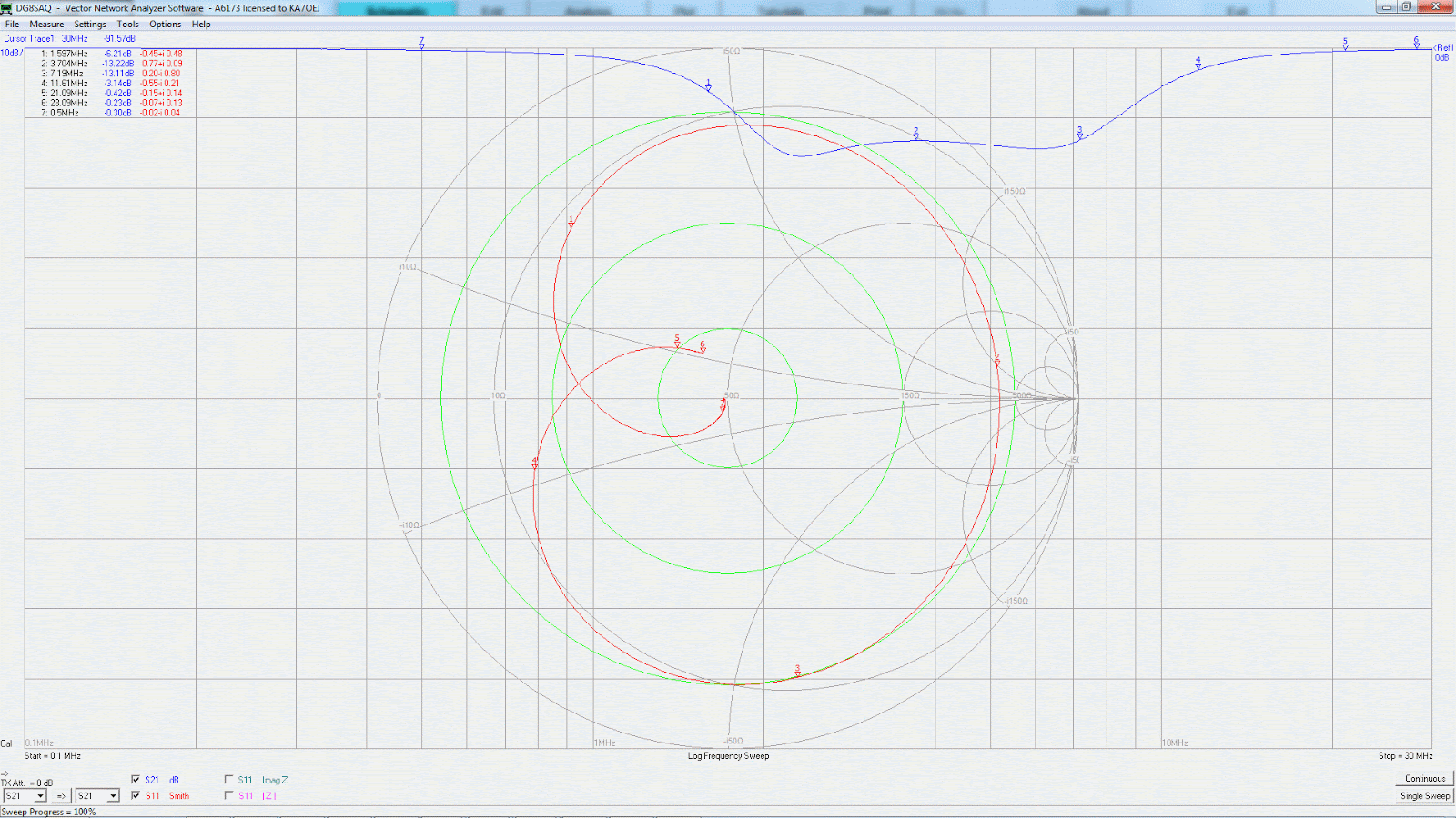
• As can be seen from the Smith chart in Figure 2, this filter provides a 50 ohm match only at frequencies removed from the portion where the attenuation is occurring.  For this reason it is recommended that this filter be placed fairly close to the receiver (or splitter, if several receivers are being used) - this, to prevent impedance transformation on the line.  Similarly, it is recommended that this filter be preceded one stage of amplification to source the filter with something near-ish 50 ohms.
• If amplification is used for the receiver, it is suggested that the bulk of amplification be placed immediately after this filter:  The attenuation at the lower frequencies will reduce the probability of amplifier overloaded by the often-strong signals at these frequencies as well as the summer static.  The impact of the filter on the system noise figure at low frequencies is offset by the typically-high noise level while the low loss of the filter at higher frequencies which means that there will be little overall impact at the high end of the HF spectrum.
• In the case of the KiwiSDR system at the Northern Utah WebSDR, the total amount of amplification is about 22 dB in two stages:  At least 10dB is required in the overall system just to bring the receiver's noise floor (at 30 MHz) below the "rural quiet" noise floor - and there are likely to be other system losses that require even more amplification.  At the Northern Utah WebSDR, there is about 5 dB of loss between the antenna and the first amplifier, and there is an additional 6.5-7dB of loss in a four-way splitter to feed all of the receivers, so the overall 22dB gain in the system is about right.

This page stolen from ka7oei.blogspot.com

[End]

A limited attenuation high-pass filter for the KiwiSDR

NOTE:

Figure 1:
Inside the "limited attenuation" high pass filter, housed inside a small, die-
cast aluminum enclosure to which two BNC connectors were mounted.  Some
components were secured using small dabs of clear RTV sealant.
Click on the image for a larger version.

There is a follow-up articles to this one that describes a circuit that properly matches the source/load over a wide frequency range - See the article: "Revisiting the limited attenuation high-pass filter for the KiwiSDR" link and  "Revisiting the limited attenuation High Pass Filter - again".

 

Since the original posting of this blog entry I was made aware of an 1977 article on this very topic - you can read it HERE. (The article in question begins on page 3 of the PDF.)

* * *

One of the issues common with using a broad-band, direct-sampling SDR (software-defined radio) like the KiwiSDR is that of overload by strong, low-frequency signals, such as those on the AM (mediumwave) broadcast band - but there's another problem that should be considered as well:  The high generally-high signal levels at lower HF frequencies.  If one looks at an spectrum analyzer connected to a broad-band receive  antenna during the evening, one will immediately note that the lower the frequency, the higher the signals seem - particularly the background noise.

This becomes problematic if one is using an antenna with a relatively flat gain across the entire HF spectrum - and one wishes to make the receiver usable at both the top and bottom ends of this range.  As an example, I have a KiwiSDR connected to an antenna that is rated to cover from 3 to 30 MHz with roughly constant gain, but I noted that at the top end of the frequency range, around the 10 meter amateur band, the overall system gain was not quite sufficient to "hear" the background iononspheric noise.

The obvious solution to this gain deficit is to install an RF amplifier - which I did - but this had the effect of increasing the already-strong signals below 5-10 MHz even more, resulting in occasional "OV" indications on the KiwiSDR's S-meter signalling to me that the RF levels were high enough to "clip" the A/D converter.  While this wasn't too much of a problem during normal conditions, if the lower HF band were particularly noisy - as often occurs in the summer with thunderstorms on the same continent - reception across the entire HF spectrum was compromised when the loud static crashes would occasionally saturate the A/D converter.

It occurred to me that while I had about the right amount of system gain on 10 meters, I had far more than I needed at lower frequencies and could throw some of it away, so I set about designing a filter that would reduce signals at the low end of the HF spectrum, but have minimal effect at the upper end.

A "limited" high-pass filter:

Note:  The filter detailed below is NOT recommended as it does not match well to 50 ohms across Ll frequencies - see the follow-up article HERE for one that provides a good match/return loss.

 
The obvious solution to this would be the addition of a high-pass filter - but there's a problem:  Even a minimal high-pass filter would have increasingly-higher attenuation at lower and lower frequencies - potentially in the many 10s of dB - but we don't really want to get rid of the lowest frequencies.  What we need is a filter that will "knock down" signals by a significant amount - but not so much that they become inaudible.

In analyzing the signal levels, I determined that the goal of the design would be to leave signal levels above about 10 MHz unaffected, but reduce the signals below 8 MHz or so by 10-15dB.  This amount of attenuation (about 2 "S" units) would significantly reduce the amount of RF energy entering the A/D converter at the lower end of the frequency range (about 2 "bits" worth) but analysis of the noise floor and signal levels at these lower frequencies indicated that I would still be able to hear the noise floor.

The diagram of this filter is shown below:

Figure 2:  Diagram of the "limited attenuation" 10 MHz high-pass filter.
This filter attenuates by about 12dB (2 "S" units) below 8-10 MHz, reducing the overall signal power reaching the A/D converter of the KiwiSDR.
"R2" represents the 50 ohm input of the receiver and is not a resistor.
See text below for details of L1-L4.

The diagram above, as rendered by "LT Spice", depicts the load (the receiver) as R2, a 50 ohm resistor - and this is not an actual component that would be installed.

No real attempt was made to make this filter's input and output impedances "flat" across the entire HF spectrum - and to be sure, below about 14 MHz its input impedance a bit high, but this will have little practical effect on its operation - and we really don't need to be too precise, anyway.

As tested on a spectrum analyzer, the insertion loss is 12-13dB from DC to about 4 MHz at which point it gradually drops to about 2dB at 11 MHz and then dropping to less than 1dB by 30 MHz.  When doing an "A/B" comparison with and without the filter on the KiwiSDR, the waterfall above 10 MHz looked unchanged, but the signals below about 7 MHz were much less "bright" - and most importantly, the occasional "OV" indications on the S-meter pretty much stopped appearing altogether.

Comment:

In my opinion, the RF input on the KiwiSDR is slightly deaf, requiring a bit of gain (say, 6-10dB) to be able to reliably hear the background ionospheric noise on the higher HF bands - particularly when they are closed - a problem compounded by normal amplitude roll-off as one nears the Nyquist frequency.  To this end, the KiwiSDR at this location is preceded by a low-noise, high dynamic range RF amplifier that is flat from a few 10s of kHz to well over 30 MHz.

Update:

After this article was originally written it was determined by several testers using different KiwiSDRs that the absolute sensitivity of a KiwiSDR is on the order of -155dBm/Hz for 0dB S/N at 28 MHz.  This sensitivity level is about 6-8 dB below the expected noise at a "quiet" site using a unity gain antenna on the 10 meter band.

In the real world, it is likely that 10-12 dB of overall signal amplification should preceded a KiwiSDR to allow it to be sensitive enough to hear the noise on a "quiet" 10 meter band and the weakest signals.  If amplification is used, it should be placed as close to the antenna as possible in the signal path, but after a filter such as that described on this page (the filter will reduce the probability of overload by strong signals below 10 MHz and its loss at 10 meters is low and will have minimal effect), and before any splitter if you plan to feed more than one receiver from that signal path.  When the overall amount of amplification is calculated, be sure to include the loss of a splitter is taken into account.  For example, a 4-way splitter will incur about 7dB of loss, so if you wish the KiwiSDR to "see" 12dB of additional signal at 10 meters you will need an amplifier with a gain around 20dB.

The components for construction of this filter aren't critical:  The capacitors are high-stability NP0 (a.k.a. C0G) ceramic types while L1-L3 are wound using 30 AWG enameled wire with L1 and L2 having 15 turns and L3 having 12 turns on T37-2 toroidal cores, respectively.  L4 is a an inexpensive molded inductor and its value can be anything from 2.2 to 3.3 uH, or one could make it by winding 25 turns on the same type of T37-2 toroidal cores as used for L1-L3.

A look at the Kiwi's waterfall with the filter:

Figure 3, below, shows this filter in place on the KiwiSDR at the Northern Utah WebSDR site:

Figure 3:
A 1-18 MHz span of the waterfall from a KiwiSDR with the "limited attenuation" high-pass filter.  At the far left side a mass of signals from local AM broadcast stations can be seen.
The horizontal streaks are from wideband lightning static that is slightly "noising up" the A/D converter in the KiwiSDR.
Click on the image for a slightly larger version.

If you look at the waterfall above, there's no obvious evidence of the filter described on this page even being connected - and that's exactly the point!  The only evidence that something is a bit "strange" is the fact that the background noise between 8 and 11 MHz is slightly higher - and that's exactly where the filter rolls off:  At increasingly higher frequencies in this range, the natural noise drops off a bit - but the filter doesn't drop off at quite the same rate with the result being that the overall signal levels in this range are slightly elevated.

If I build another of these filters I'll push the "knee" up 1-2 MHz higher, starting the roll-off of signals below 11-12 MHz, instead.

Conclusion:

This filter seems to be very effective in reducing the total signal power from lower HF frequencies while having minimal effect at higher frequencies.  Because the signal+noise levels from a broadband antenna are much higher at the lower end of the spectrum, it is possible to reduce these signals by 2 "S" units or so without dropping the background noise - or the signals themselves - below the noise floor of the receiver.

For information on a filter system that is specifically designed to attenuate AM (MW) broadcast band signals, see the article "Managing HF signal dynamics on the RTL-SDR (and KiwiSDR) receivers", also on this blog.

Follow up:

There is a follow-up article to this one - "Revisiting the limited attenuation high-pass filter for the KiwiSDR" link where a variation of this filter is presented that passes the AM broadcast band and frequencies below it and is recommended for those installation where you wish to receive longwave signals.

[End]

This page stolen from ka7oei.blogspot.com