Characterizing spurious (Harmonic) responses of the SDRPlay RSP1a (and other models)

The SDRPlay RSP2pro (left) and RSP1a receivers (right)

The SDRPlay RSP1a is a popular Software Defined Radio (SDR).  This device, connected to and powered by the computer via a USB cable covers from VLF through UHF and low microwave frequencies.

This receiver shares a similar internal architecture of similar devices such as the RTL-SDR dongle and the AirSpy in that an analog frequency converter (mixer) precedes the analog-to-digital converter:  In the case of the SDRPlay, the frequency to which the receiver is tuned is (usually) converted to baseband I/Q signals, with the "center" frequency being at zero Hz (DC). ¹

Note:

For the purposes of this discussion, there is no difference between the RSP1a and some of the other receivers in the product lineup (e.g. RSPDuo, RSPdx and the discontinued RSP1, RSP2 and RSP2pro) in terms of harmonic response across the 2-30 MHz range as they all have about the same 12 MHz and 30 MHz cut-off frequencies on their input filtering - properties that would affect HF reception across the 2-30 MHz range in terms of harmonic response.

This issue was noted at least as far back as 2017 in the SDRPlay forum - See this thread:  https://www.sdrplay.com/community/viewtopic.php?t=2280

Imperfect mixers

By its nature, a frequency mixer is a non-linear device.  Ideally, the two frequencies applied to a mixer would yield just two more - the sum and difference.  For example, if we applied a 5 MHz signal and a 1 MHz signal to a mixer, it would output both the sum of 6 MHz and the difference of 4 MHz - and this is true, but there's more to the story.

In our example - with a real-world mixer, we will also get additional products - including those related to the harmonics of the local oscillator and the applied signal.  Because of this, we will see weaker signals at:

• 11 MHz (2 * 5 MHz + 1 MHz) 
• 9 MHz (2 * 5 MHz - 1 MHz) 
• 7 MHz (5 MHz + 2 * 1 MHz) 
• 3 MHz (5 MHz - 2 * 1 MHz) 
• And so on.

Typically, these "other" signals will be quite a bit weaker than the original - but they will still be present, possibly at a high enough level to cause issues such as spurious signals - a problem with both receivers and transmitters.  Typically, these are tamed by proper design of the mixer, proper selection of frequencies and careful filtering around the mixer to limit the energy of these "extra" signals.

Note:  There will be a response at 5x the center frequency as well, but it is suppressed better than the 3x response by the mixer and - for the 80 meter amateur band and higher - these responses are suppressed reasonably well by the filtering.

SDRPlay's poor harmonic response suppression on 80 meters and below.

ANY receiver will experience spurious responses related to mixing products.  Typically, filtering is employed to remove/minimize such responses, but for a wide-bandwidth receiver such an SDR, doing this is complicated by the fact that being able to cover wide swaths of bandwidth would ideally require a large number of overlapping filters.

An example of a radio where this is done - albeit of different architecture - is the Icom IC-7300 which has nine overlapping band-pass filters that cover 160 through 10 meters.  While the reasons for the '7300 having many filters has as much to do with its being a "direct sampling" ² type of SDR, good filtering on the signal path of any type of receiver - SDR or "HDR" (Hardware Defined Radio - or an "old school" analog type) is always a good idea

If this many filters had been implemented on the SDRPlay, there would be enough filtering to prevent a significant harmonic response.  In the case of the RSP1a, this was not done - partly to allow 5-8 MHz of continuous coverage without being significantly impacted by the filters in many cases, but more likely it was done due to practical reasons of economics ³ :  There are just three filters used for covering all of the "HF" amateur bands 160 through 10 meters:  One that covers up to 2 MHz, another that covers 2-12 MHz and third that covers 12-30 MHz:  This information is covered in the RSP1a technical information document ( https://www.sdrplay.com/wp-content/uploads/2018/01/RSP1A-Technical-Information-R1P1.pdf )

The sensitivity to harmonics was tested with the RSP1a's local oscillator (but not necessarily the virtual receiver) tuned to 3.7 MHz ⁴ .  For reasons likely related to circuit symmetry, it is odd harmonics that will elicit the strongest response which means that it will respond to signals around (3.7 MHz * 3) = 11.1 MHz.  "Because math", this spurious response will be inverted spectrally - which is to say that a signal that is 100 kHz above 11.1 MHz - at 11.2 MHz - will appear 100 kHz below 3.7 MHz at 3.6 MHz.  (It's likely that there are also weaker responses at frequencies around 5 times the local oscillator, but these are - for the most part - adequately suppressed by the filtering.)

In other words, the response to spurious signals follow this formula:

Apparent signal = Center frequency + ((Center frequency * 3) - spurious signal) )

Where:

• Center frequency = The frequency to which the local oscillator on the RSP is tuned.  In the example above, this is 3.7 MHz.
  
• Spurious signal = The frequency of spurious signal which is approximately 3x the center frequency.  In the example above, this is 11.2 MHz.
  
• Apparent signal = Lower frequency where signal shows up.   In the example above, this is 3.6 MHz.
  

In our example - a tuned frequency of 3.7 MHz - the 3rd harmonic would be within the passband of the 2-12 MHz filter built into RSP1a meaning that the measured response at 11.2 MHz will reflect the response of the mixer itself, with little effect from the filter as the 2-12 MHz filter won't really affect the 11 MHz signal - and according to the RSP1a documentation (link), this filter really doesn't "kick in" until north of 13 MHz.

In other words, in the area around 80 meters, you will also be able to see the strong SWBC (Shortwave Broadcasting) signals on the 25 meter band around 11 MHz.

How bad is it?

Measurements were taken at a number of frequencies and the amount of attenuation is indicated in the table below.  These values are from measurement of a recent-production RSP1a and spot-checking of a second unit using a calibrated signal generator and the "HDSDR" program:

LO Frequency	Measured Attenuation at 3X LO frequency	Attenuation in "S" Units
2.1 MHz	21 dB (@ 6.3 MHz)  - Using 2-12 MHz filter	3.5
2.5 MHz	21 dB (@ 7.5 MHz)	3.5
3.0 MHz	21 dB (@ 9.0 MHz)	3.5
3.7 MHz	21 dB (@ 11.1 MHz)	3.5
4.1 MHz	23 dB (@ 12.3 MHz)	3.8
4.5 MHz	30 dB (@ 13.5 MHz)	5
5.0 MHz	39 dB (@ 15.0 MHz)	6.5
5.5 MHz	54 dB (@ 16.5 MHz)	9
6.0 MHz	54 dB (@ 18.0 MHz)	9
6.5 MHz	66 dB (@ 19.5 MHz)	11
12.0 MHz	21 dB (@ 36.0 MHz) - Using 12-30 MHz filter	3.5
12.5 MHz	21 dB (@ 37.5 MHz)	3.5
13.5 MHz	22 dB (@ 40.5 MHz)	3.7
14.5 MHz	26 dB (@ 43.5 MHz)	4.3
15.5 MHz	31 dB (@ 46.5 MHz)	5.2
16.5 MHz	35 dB (@ 49.5 MHz)	5.8
17.5 MHz	39 dB (@ 52.5 MHz)	6.5
18.5 MHz	43 dB (@ 55.5 MHz)	7.2
19.5 MHz	46 dB (@ 58.5 MHz)	7.7
20.5 MHz	50 dB (@ 61.5 MHz)	8.3
21.5 MHz	53 dB (@ 64.5 MHz)	8.8

Table 1:  Measured 3rd harmonic response of the RSP1a

Interpretation:

• In the above chart we see the local oscillator frequency in the left column, the measured attenuation of the 3rd harmonic response (and its frequency) in the center column, and that amount of attenuation expressed in "S" units.  Here, an "S" unit is based on the IARU standard (Technical recommendation R.1) of 6 dB per S unit, which is reflected in programs like SDRUNO, HDSDR and many others.
  
• The attenuation of the 3rd harmonic response was measured by first noting the signal level required to obtain a given reading - typically "S-9" near the fundamental frequency - and then observing the level required to obtain that same reading - within +/-1dB - near the 3rd harmonic frequency, using the relationship formula, above.
  
• Below the cutoff frequency of the relevant filter (nominally 12 MHz for receive frequencies in the range of 2 to 12 MHz, nominally 30 MHz for receive frequencies in the range of 12 to 30 MHz) the harmonic response is limited to that of the mixer itself, which is about 21 dB.
  
• We can see that on the 2 to 12 MHz segment, the attenuation related to the 3rd harmonic doesn't exceed 40 dB (which is the low end of what I would call "OK, but not great) until one gets above about 5 MHz (which translates to 15 MHz) and it doesn't get to the "goodish" range (50dB or more) until north of about 5.5 MHz which is borne out by the filter response charts published by SDRPlay.
• On the 12 to 30 MHz band the 2-12 MHz filter has practically negligible effect until one gets above about 20 meters, at which point it gets into the "OK, but not great" range by about 18 MHz, and it doesn't really get "goodish" until north of 20.5 MHz.
• Similarly, the "12-30 MHz filter isn't particularly sharp, either.  What this means is that strong 6 meter signals may well appear in the 16.5 to 17.5 MHz range as frequency inverted representations.
• If there is a relatively strong signal source in the area of the 3rd harmonic response, it will likely appear at the lower receive frequency where the attenuation of the filter is less than 40 dB or so.  The severity of this response will, of course, depend on the strength of that signal, the amount of attenuation afforded by the filters at that frequency, and the amount of noise and other signals present in the range of the fundamental frequency response.
  

Based on the above data, we can deduce the following:

• When the RSP1a is tuned between 2 MHz and (below) 12 MHz, it is using its "2-12 MHz" filter. In this range - and below approx. 4 MHz - the 12 MHz cut-off of the filter has negligible effect in reducing 3rd harmonic response.
• What this means is that signals from 6-12 MHz will appear more or less unhindered (aside from the 21 dB reduction afforded by the mixer) when the local oscillator of the receiver is tuned between 2 and 4 MHz.
• The 3rd harmonic response across 2-4 MHz - which is the 6-12 MHz frequency range - can contain quite a few strong signals and noise sources such as those from shortwave broadcast stations.
  
• When the RSP1a is tuned between 12 MHz and (below) 30 MHz, it is using its "12-30 MHz" filter.  Below about 14 MHz, the 30 MHz cut-off of the filter has negligible effect in reducing 3rd harmonic response.
• Signals from 36-40 MHz will appear with just 21-26 dB attenuation when tuned in the range of 12-13.5 MHz.
• In most cases there are probably few signals in the 36-40 MHz range that are likely to be an issue when tuning in the 12-13.5 MHz range.

80 meter example:

Connecting the RSP1 to a known-accurate signal generator set to -40dBm, the signal level at 3.6 MHz was measured:  Maintaining the signal level, the generator was retuned to 11.2 MHz and the resulting signal level was measured to be 21 dB (a bit more than 3 "S" units) lower than that at 3.6 MHz.

What this means is is that a "20 over S-9" signal at 11.2 MHz will show up as an S-9 signal at 3.7 MHz, and an S-9 signal at 11.2 MHz will be around S-6 at 3.7 MHz.  In other words, even a "weak-ish" signal at the 3rd harmonic will show up at the lower frequency.

80/60 meter example:

If you run the RSP1a in a wider bandwidth mode, it is possible to simultaneously see and tune a greater frequency range.  For example, let us presume that you wish to cover both 80 and 60 meters using a single RSP1.  To do this, you could set the center (LO) frequency to 4.5 MHz and set the sample rate to 5.376 MHz and use the 5 MHz band-pass filter built into the RSP1's converter/mixer chip (the Msi001) to prevent in-band aliasing.

In this configuration 20 meter signals will appear at the top of 80 meters owing to the relationship in the formula that we described above.  Taking the 20 meter FT-8 subband at 14.074 MHz as an example, we see that:

4.5 MHz + ((4.5 MHz * 3) - 14.074) = 3.926 MHz

In other words, we will see spectrally-inverted representations of 20 meter FT-8 signals around 3.926 MHz, and the rest of the (upper) portion of 20 meters across the rest (lower) portion of 80 meters where USB signals on 20 meters will show up as LSB signals on 80.  We know from the chart above that those signals will be attenuated by between 30 and 39 dB (about 5-6 S-units).  This might sound like a lot of attenuation, but it means that a "20 over" signal on 20 meters will appear at around S-7 to S-8 on 80 meters - still quite respectable most certainly very audible!

More about filtering and harmonic response

While these spurious responses may not be too much of a problem for the casual user, it will be necessary to add additional filtering to allow the RSP1a to function on par with a modern, SDR receiver from one of the major manufacturers.

Unfortunately, the filtering in the RSP1a is not sufficient in the 80 meter case mentioned above as it doesn't have octave filters (or similar) - but what about 60 or 40 meters?

The table above answers this question.  In the case of 60 meters - with the receiver tuned to 5.3 MHz - our 3rd harmonic will land on 15.9 MHz.  Based on measurements of the receiver the response of signals around 15 MHz - which corresponds to the 19 meter Shortwave Broadcast Band - will be a bit more than 40 dB down from 40 meters with about 20 dB of this being due to the roll-off of the 2-12 MHz filter - but because this frequency range is inhabited by very strong shortwave broadcasters they are likely to still be quite audible around 60 meters.

The situation is a bit better for 40 meters where the 3rd harmonic is around the 15 meter band.  There, the 2-12 MHz filter knocks signals down by 50dB or more, putting them about 70dB below the 40 meter response - on par with about any respectable receiver.

What this means is that for amateur bands below 40 meters it is suggested that additional filtering be applied.

The best solution - and recommended for any software-defined radio (or even older "hardware-defined radios") is to have band-pass filter designed for the specific amateur band in question. This will not only significantly attenuate the harmonic response, but it will also reduce the total amount of RF energy entering the receiver, reducing the probability of overload.  The obvious down-side is that it will reduce the flexibility of the receiver in that unless you change/remove it, you won't be able to receive signals well outside the filter's design range.

Another possibility is to add a low-pass filter that is designed to cut off signals above the band of interest.  For example, if you have a filter that cuts off sharply above 8 MHz, you will be able to tune 80-40 meters and get reasonable attenuation of the 3rd harmonic response across this entire frequency range.

In the case of 160 meters the RSP1a will automatically select the 0-2 MHz low-pass filter and the 3rd harmonic response will be a respectable 50-ish dB down, depending on frequency.

On 20 meters - where the 3rd harmonic is around 42 MHz - the "12-30 MHz" filter will be selected, but the published response of this filter shows that at 42 MHz its attenuation will be quite limited.  Practically speaking, it is unlikely that there will be any signals in this frequency range so there being "only" 20-30dB of attenuation is unlikely to cause a problem in most cases, but one should be aware of this.

What can be done:

In short, none of the currently-made SDRPlay receivers - by themselves - will offer very good performance in terms of harmonic rejection between 2 and 5 MHz and it will be particularly bad on the 80 meter band where strong 25 meter SWBC signals can appear:  It is interesting that the ARRL review of the RSPdx (Link here) didn't catch this issue.

It is unfortunate that the designers of the SDRPlay receivers did not add at least one additional low-pass filter in the signal path to quash what is a rather strong response in the 2-6 MHz range - particularly on 80 meters, one of the most popular bands.  A low-pass filter with a cut-off frequency of 6 MHz (with attenuation becoming significant above 7 MHz) would ameliorate the harmonic response when tuning across this band.  This problem is made even worse by the fact that even antennas that aren't particularly resonant at their harmonic responses (e.g. the antenna for 80 meters) will likely do quite a decent job of receiving signals in the 11-12 MHz area.

The only real "fix" for this is to install additional filtering between the SDRPlay receiver and the antenna.  If single-band operation is all that is desired, the best choice will be a band-pass filter designed for the frequency range in question ⁵ - but unless you are dedicating the receiver just for that one band, this isn't really desirable unless you can easily switch/bypass the filter when tuning elsewhere.

A more flexible solution would be to use a low-pass filter.  As we noted above, the 12 MHz roll-off of the built-in (2-12 MHz) filter just doesn't do much to suppress signals from 20 meters, but if we had a filter that had a sharp cut off beginning, say, at 8 MHz, we could use it for 80, 60 and 40 meters - such a filter is depicted schematically, below:

8 MHz low-pass filter schematic, designed using ELSIE

This filter is pretty easy to build:

• Capacitors 1 and 5 each consist of a 100pF and 470pF in parallel
• Capacitor 3 consists of a 680pf and 220pF in parallel - although you could probably get away with two 470pF capacitors in parallel in a pinch.
  
• Inductors 2 and 4 consist of 16 turns on a T50-2 (or 18 turns on a T37-2) toroid using small wire - 24-30 AWG (0.6-0.25mm dia.) is fine

A small scrap of PC board material - about 2"x4" (5x10cm) is more than large enough to accommodate with the capacitors soldered directly to the foil and inductors held aloft by the capacitors.  The connectors should be attached to the PC board directly - or with short lengths of coax, keeping the ground (shield) lead length to an absolute minimum to minimize the probability of ground-loop induced noise currents.

If you have access to a NanoVNA it's quite easy to check the performance.  If anything, it may be necessary to spread the turns across the toroid or remove one turn - but this design is quite forgiving and it should work adequate with no tuning at all.

The obvious down-side for this is that if you are tuning all over the HF spectrum (above 7.5-8 MHz in the case of the filter above) you'd have to manually remove or bypass any such filtering when you tuned beyond the range that the added filter would pass.

 

Footnotes:

1. The receivers mentioned at the beginning of the article (SDRPlay, AirSpy HF, RTLSDR, etc.) have analog-to-digital converters that cover only a portion of the HF spectrum, using a frequency mixer to convert a range of frequencies from the range of interest to a lower frequency, which is then fed into the converter.  Limiting the amount of spectrum being ingested by the receiver - particularly when appropriate filtering is used - can improve performance, reduce cost, and especially reduce the total amount of data, allowing a modest computer (older PC, Raspberry Pi) to be used with it.
   
2. A "direct sampling" type of receiver - such as that found in the Icom IC-7300, IC-7610, the KiwiSDR, Red Pitaya and the RX-888 (when used at HF) and others like them simply "inhale" large swaths of spectrum all at once.  Because the analog-to-digital converter itself has a limited amount of total RF signal power that it can handle, radios like the Icoms have filtering that allow the passage of only the (relatively) small portion of the HF spectrum around that to which the receiver is tuned, reducing the probability of overload from strong signals on frequencies well away from those of interest.  Other direct-sampling receivers such as the KiwiSDR, Red Pitaya and RX-888 do not necessarily have band-specific filtering as they are intended to be able to receive multiple frequencies across the entire HF spectrum at once and as such, much more care is required in implementation to prevent overload/distortion for these devices.
   
3. In the case of the (currently-produced) RSP receivers, the filtering varies depending on model:  In the case of the RSP1a, it has a band-pass filter that covers 2-12 MHz while other models have used just a 12 MHz low-pass - the former being capable of rejecting AM broadcast band (e.g. mediumwave) signals from the input of the receiver when tuned to HF, and the latter not.  Some units additionally have a separate "notch" (reject) filter that is designed to remove just AM broadcast-band signals.  The situation described in this article - the reception of signals around 11 MHz when tuned to 80 meters - is related to the fact that the 2-12 MHz filter represents a 6:1 frequency range which means that over the lower portion of this spectrum, the 12 MHz cut-off of this filter cannot possibly remove responses to the third harmonic, hence the issue described here.
4. If you are using a program like SDRUno it may not be readily apparent to what frequency the receiver's local oscillator is tuned.  If set to "Zero IF" mode, the local oscillator will be tuned at the same place as the center of the waterfall display when it is fully zoomed out - typically indicated by a slight line at the "Zero Hz" frequency there there is a slight amount of noise energy.  By default, one cannot directly tune the local oscillator ("Zero IF" frequency) in SDRUno.  If you use the "HDSDR" program by I2PHD (et al) you can independently tune the local oscillator and the frequency of the virtual receiver.
   
5. SDRPlay receivers are currently in use at a number of well known and public WebSDRs around the world as the "acquisition device" (e.g. receiver).  In most cases these receivers - because they are used only for specific amateur bands - are preceded by a band-pass filter for the band that they are covering, completely eliminating issue noted in this article.  It was during testing at one of these WebSDRs - a receiver on 80 meters that does not (yet) have additional filtering - that signals were noted across the 80 meter band in the middle of the day that should not have been there at all - and these signals were quickly realized to be the result of a harmonic response in the front end.  These responses were then verified and quantified using two other RSP1a receivers (of different production runs) and test equipment during the preparation of this article.  When it was convenient to do so, a low-pass filter with a cut-off frequency of 7.5 MHz was installed on this receiver, solving the image problems.
   

* * *

This page stolen from ka7oei.blogspot.com

[End]

Revisiting the "Limited Attenuation High Pass" filter - again.

In several previous posts (See:  "A Limited Attenuation High Pass Filter" and "Revisiting the Limited Attenuation High Pass Filter" I described a "high pass" filter that offered low attenuation at high HF frequencies, but a controlled amount of attenuation at lower frequencies - this, to accommodate a fundamental fact about both HF propagation and direct-sampling Software Defined Radios (SDRs):  The two don't play nice with each other!

Note:

If you are using any direct-sampling Software Defined Radio to receive ALL of the HF spectrum simultaneously  - such as a KiwiSDR, Red Pitaya, RX-888, RX-666, TRX Duo to name but a few - you SHOULD read this page and understand why it is important to apply such filtering to maximize performance across HF.

In a typical receiver/antenna configuration, failure to reduce the lower HF frequencies with respect to the top of the HF spectrum (e.g. 10 meters) will result in comparatively poor performance.

As noted in the previous post(s), the problem is two-fold when it comes to broad-band SDRs that are intended to cover the entire HF spectrum all at once:

• HF noise power and signal level is (generally) inversely proportional to frequency.  At lower frequencies - say, 2-8 MHz - the noise power is far higher than it typically is at around 20-30 MHz.

• A direct-sampling SDR - or any receiver, for that matter - can tolerate only so much RF power on its front end.  Traditionally, this is a mitigated with the use of narrow-band RF band-pass filters, but this can't be done if one intends to be able to cover the amateur radio bands 160 through 10 meters (1.8-30 MHz).

With the aforementioned issues is yet another one:  Because the noise floor at 10 meters when it is "quiet" is so much lower than 80 meters (perhaps 40-50 dB during noisy nighttime conditions, 25 dB or so during quiet daytime conditions) there is an intrinsic disparity between the amount of sensitivity that is need to "hear everything" at the opposite ends of of the HF spectrum - but since a typical direct-sampling SDR is pretty much "flat", we end up with what might seem like a pair of intractible problems:

•  To accommodate the very strong signals and high noise levels at lower HF frequencies, the RF signal gain in front of the A/D converter must be carefully set to prevent overload.

• In order to "hear" the noise floor at 10 meters, the system gain must be set fairly high.

What these two factors, together, imply is that if we have enough gain to comfortably detect the noise floor at 10 meters, our receiver will be badly overloaded during strong-signal conditions on the lower bands.  Conversely, if we scale (e.g. attenuate) the input to accommodate the very large signal excursions, the receiver will simply be unable to detect signals at/near the "quiet" 10 meter noise floor.

Comments:

There will (hopefully) be the day that the upper HF propagation conditions improve greatly with the arrival of solar cycle 25 and at that time, strong signals will appear on the bands >=15 MHz.  When this happens, we will likely be faced with a problem similar to that which we are trying to solve here (e.g. very strong signals overloading the A/D converter).  At this time, the only recourse will likely be a means of using an external device to adjust the gain/attenuation in front of the receiver, probably using the existing I/O lines under receiver control.

Since the original posting of this blog entry I was made aware of an 1977 article on this very topic - you can read it HERE. (The article in question begins on page 3 of the PDF.)

A revised circuit:

Why talk about this issue a THIRD time?  I decided to make one that provided a better 50 ohm match across all frequencies than the previous versions.  This revised circuit may be seen in the figure below:

Figure 1:
Generic pre-emphasis network set for about 50 ohms.
Click on the image for a slightly larger version.

Some readers will recognize the topology of the circuit in Figure 1 as the classic pre-emphasis network found in the signal  path of FM video transmitters.  Whereas those circuits are typically designed for 75 ohms, this one is intended for a 50 ohm system - but careful observers will notice that 47 ohm resistors are used, instead:  For receive-only purposes, I have chosen the components in this article to be standard values at the expense of a slight increase in mismatch - but the VSWR of these circuits, when terminated at 50 ohms - is likely to be no more than about 1.1:1.

This circuit - compared with the previous versions - has the advantage that it presents a consistent source and load impedance across the frequency range, making it a bit more "friendly" in systems that may be impedance sensitive (e.g. following a band-pass filter, long coaxial cable runs, following/preceding conditionally-stable RF amplifiers.)  The obvious trade-off is that as compared to the previous version (which was based on a high-pass filter and some resistive bypassing) this circuit has definite limitations on how sharp and deep the "knee" may be at any given frequency as only a single inductor and capacitor are used.

By tweaking the values of R1, R4, C1 and L1 we can adjust both the amount of low-frequency attenuation and the frequency of the "knee" where the attenuation takes place - but for our purposes, we will be placing the center of that "knee" around 10 MHz to provide both the minimal loss at 30 MHz and adequate attenuation at and below 7 MHz.

Here are a few examples of values of R1, R4, C1 and L1 using standard-value components and approximate attenuation values at various frequencies:

R1 = 68 ohms  R4 = 39 ohms C1 = 390pF  L1 = 1uH DC attenuation:  7.3dB @ 2 MHz: 7.0dB  @4 MHz: 6dB @ 7 MHz: 4.6dB  @10 MHz: 3.4dB @ 14 MHz: 2.3dB  @28 MHz: 0.8dB	R1 = 120 ohms  R4 = 20 ohms C1 = 330pF  L1 = 0.82uH DC attenuation:  10.8dB @ 2 MHz: 9.8dB  @4 MHz: 8.1dB @ 7 MHz: 5.6dB  @10 MHz: 3.9dB @ 14 MHz: 2.5dB  @28 MHz: 0.8dB
R1 = 120 ohms  R4 = 20 ohms C1 = 270pF  L1 = 0.68uH DC attenuation:  10.8dB @ 2 MHz: 10.1dB  @4 MHz: 8.7dB @ 7 MHz: 6.5dB  @10 MHz: 4.8dB @ 14 MHz: 3.3dB  @28 MHz: 1.2dB	R1 = 100 ohms  R4 = 27 ohms C1 = 270pF  L1 = 0.68uH DC attenuation:  9.4dB @ 2 MHz: 8.9dB  @4 MHz: 8dB @ 7 MHz: 6.3dB  @10 MHz: 4.8dB @ 14 MHz: 3.6dB  @28 MHz:1.3dB

Figure 2:
Table showing some possible values for the circuit of Figure 1 and the example attenuation values.

 

In practice, several of these sections will likely need to be cascaded to achieve the desired amount of attenuation at the lower HF frequencies which brings up the question:  Could you not choose components to do this for a single section?  The answer is theoretically, yes - but the fact is that practical inductors - particularly the molded type - are quite lossy, departing from the intended attenuation curve, and achieving the predicted, higher amount of lower-frequency attenuation with a single stage can become problematic - so it's probably better to cascade several of these networks together, instead.

A practical example:

Figure 3:
The exterior of the four channel filter network.
Click on the image for a larger version

A practical example of such a network is one that is to be currently installed in the KFS (Half Moon Bay, CA) KiwiSDR/WSPRDaemon system.  There, four wideband antennas are available to feed the KiwiSDRs on site, so a box was constructed with four, identical pre-emphasis networks, each to feed its own receiver stack.

As is the case at the Northern Utah WebSDR, noise and signals at the lower end of the HF spectrum is often very much stronger than at the high end:  If amplification is added to allow the detection of the noise floor at 10 meters, there is the very high probability that the receiver will badly overload on HF signals from the lower end of the spectrum.

Each "channel" of the device depicted in Figure 3 is identical, consisting of two cascaded sections.  The first section is that from the upper-left quadrant of the table (R1=68 ohms, C1 = 390 pf) and the upper-right quadrant (R1=120 ohms, C1 = 330pF).  Rather than the use of molded chokes, the individual inductors were wound using 30 AWG wire on T25-2 toroids:  17 and 15 turns for the 1 uH and 0.82 uH inductors, respectively.

Figure 4:
The interior of the four-channel network.
The circuit is simple enough to be wired "Manhattan"
style on glass-epoxy PC board material between the
two center pins of the BNC connectors.
Click on the image for a larger version

As can be seen in Figure 4, the construction is very simple, requiring no circuit board at all when using standard, through-hole components.  The circuit was built into a die-cast aluminum box with the BNC connectors holding the piece of PCB material in place.

To secure the components - particularly the small, toroidal inductors - RTV sealant (white) was used to hold components in place and to prevent adjacent wires of C1/R1 and R2/R3 from coming into contact with each other.

This method of construction is very simple and effective, offering good performance into the VHF range when reasonable care is taken.  With the 20mm high dividers between the sections installed as shown, the channel-to-channel isolation exceeded 85dB (the limit of convenient measurement) at 30 MHz.

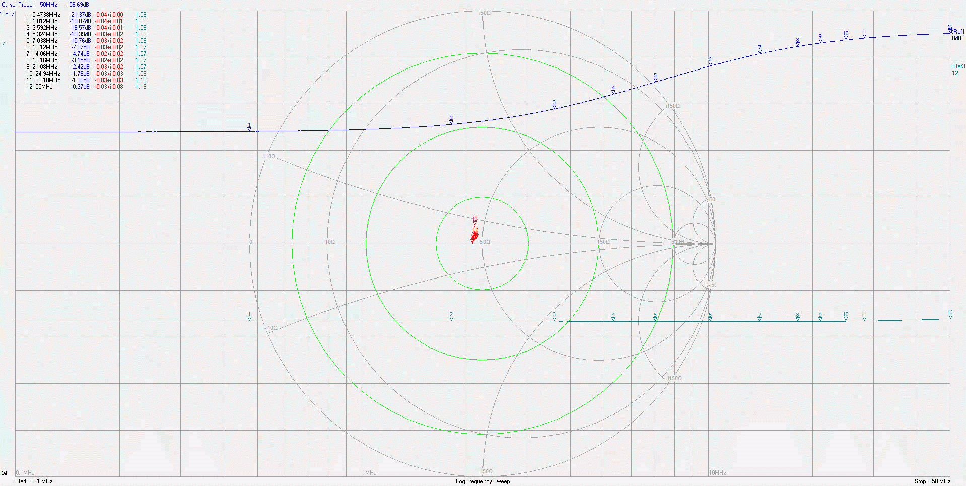
Figure 5, below, shows the typical response of the sections:

Figure 5:
The response of one of the sections as measured on a DG8SAQ VNA.
Click on the image for a larger version.

Because it can be a bit difficult to read, the values of attenuation and VSWR in the upper-left corner are reproduced below:

Frequency (MHz)	Insertion Loss (db)	VSWR
0.474	21.4	1.09
1.812	19.9	1.09
3.592	16.6	1.08
5.324	13.4	1.08
7.038	10.8	1.08
10.12	7.4	1.07
14.06	4.7	1.07
18.16	3.2	1.07
21.08	2.4	1.07
24.94	1.8	1.09
28.18	1.4	1.10
50.0	0.4	1.19

Figure 6:
Attenuation and VSWR of the network at amateur band frequencies.

 

Practical usage:

 

For large, broadband antennas and small, active E-field whip antennas, the tendency will be for a relatively "flat" frequency response - but with a small E-field whip antenna, the typical high-frequency roll-off can exacerbate the aforementioned low-HF band overload issue, making a filter network such as the above, even more indispensable.  While an attenuation value of about 17dB at 80 meters may seem to be rather extreme, unless your antenna system has severe low-frequency roll-off at the low end, the noise floor on 80 meters - even during a quiet winter day when the band is dead - should be at least several dB above the receiver's noise floor.

 For specifics relating to a wideband direct-sampling SDR like the KiwiSDR or Red Pitaya, refer to the earlier article linked above - "A Limited Attenuation High Pass Filter".

Set-up:

As mentioned above, a direct-sampling receiver like the KiwiSDR does not have enough sensitivity to "hear" the 10 meter quiet band noise floor at a very quiet receive site. In terms of overall system gain adjustment, a few comments are warranted:

• A good test is to see if, on 10 meters when it is "dead", you are hearing your local noise floor.  Note the S-meter with the antenna connected and disconnected - preferably, with the input to the receive system terminated with a 50 ohm load when disconnected.  If you do not see an increase in the S-meter reading and on the waterfall by 3-5 dB, the overall system gain is too low to allow the receiver to see the noise floor at your antenna system.
  

• If you do not see an increase in noise when the receiver is connected to an antenna, a bit of extra gain is recommended.  Given an ideal isotropic antenna at a very quiet receive site, it will probably take about 12 dB of gain to comfortably "see" the antenna's noise floor - assuming no other losses (coax, splitter, etc.)
  

• The preferred location of an amplifier is after the filter described above as it, too, will be protected against the very strong lower-frequency HF signals - even though a device like the above will increase the loss (and noise figure) by about 1.4dB at 10 meters.
  

• In cases where there are splitting losses (e.g. feeding multiple receivers) it may be beneficial to split the gain.  A modest-gain amplifier (10-14dB) might precede the splitters - the modest gain being enough to overcome splitting losses and to maintain system noise figure.
  

• In the case of a low noise level receive site, the splitting losses may put the 10 meter noise floor below the detection threshold of the receiver and, if necessary, another amplifier may be placed just after the filter described above to make up for it.
  

• It's worth noting that if you can detect a 3-5dB increase in noise floor with the antenna connected (versus disconnected) on every band, then even more gain will NOT further-improve system performance:  On the contrary, more gain than necessary will increase the probability of receiver overload - particularly on a direct-sampled SDR that has no AGC in its signal path like the KiwiSDR.  If one has more than 3-5dB of noise floor increase with the antenna connected on 10 meters when it is quiet, it's suggested that several dB of attenuation be added.  The preferred place to add this attenuation is in front of the amplifier to maximize its strong-signal handling - but only if one can still detect the noise floor on the antenna after doing so.  If one has a very high gain amplifier (say 20-25dB) and the gain is excessive, judicious addition of attenuation on both the input and output of the amplifier may be required.
  

• When an amplifier is to be considered for HF use, it should have clearly-defined ratings - one of the most important of these is the output power capability (often "P1dB" which is the output power at 1dB compression) which, for a modestly good amplifier capable of handling strong, off-air signals, should be in excess of +20dBm.  Second to this would be the 3rd order intercept point, which should be stated as being in excess of +30dBm - and the higher the better.  Both of these parameters are indicative of how well an amplifier might deal with multiple, strong signals that may be present at the antenna without adding significant distortion of its own.
  

• If you wish to pick your own frequency and impedance, the following will get you "close enough".  At the point where a single section of this circuit (as depicted in Figure 1) has an attenuation of about 4.1dB, the reactance of the "L1" and "C1" components will be equal to the desired characteristic impedance of the circuit - which will also be the same as "R2" and "R3".  Unfortunately, other parameters (e.g. the amount of attenuation at a specific frequency) are not predicted by this formula, although it's worth noting that both C1 and L1 will disappear at extremes in frequency and the circuit effectively turns into a resistive attenuator.  For example, C1 disappears (goes to infinity ohms) and L1 goes to zero ohms at DC while L1 disappears (equivalent resistance goes to infinity) and and C1 goes to zero at infinity MHz and one can pretend that these particular components no longer exist (e.g. either a short or open as appropriate).
  

Addendum:  Comments about the RX-888 (Mk2)

 

The RX-888 (Mk2) is a USB3-interfaced "signal acquisition device" - or an SDR front-end.  Unlike the aforementioned KiwiSDR, it has no signal processing capability at all - it's (more or less) just an A/D converter connected to a USB3 interface.  As such, it can operate at a sample rate of 130 MHz which means that it can acquire the entire HF+6 meter spectrum.  For various reasons (see the link below) it is usually better to operate an RX-888 at around 65 MHz, making it still-useful for inhaling the entire HF spectrum.

 

The RX-888 (Mk2) includes an attenuator (based on the PE4312) and a programmable-gain amplifier (using the AD8370) and this combination means that the noise figure PRIOR to the A/D converter will be on the order of 12 dB or so when the AD8370 is set for the "optimal" gain of about 20 dB:  See the link about signal dynamics of the RX-888 for a better explanation.  Unfortunately, the limiting factor - even with the AD8370 set for maximum gain - is the intrinsic noise of the A/D converter itself more than the components preceding it in the signal path.

 

In this case, I would make the following recommendation:

• As close to the antenna as practical, place a 10-12 dB gain, low-noise RF amplifier.  This amplifier will be the primary setting for the receive system noise figure and it should have excellent signal-handling properties.
• The "high pass filter" described above would be placed following the first amplifier.
• Following the filter, an additional 10-12 dB gain amplifier.  As the attenuation of the filter is relatively low at the frequencies where it really matters (e.g. >20 MHz) the noise figure of the receive system is preserved for these frequencies.  Placing the second amplifier downstream also reduces the total signal power that this amplifier will "see" from lower HF frequencies.  This amplifier should be chosen to have particularly handling of strong signals.
  

In the case of the RX-888, the PE4312 attenuator is likely not going to be required under any normal circumstances and should be set to "zero" and any attenuation that is needed would be set using the AD8370 amplifier.

Commercially-available version of this filter

Since this article was originally written, Turn Island Systems has produced a commercially-available version of this filter (referred to as the "shelving filter") that includes a 30 MHz low-pass filter - and you may find that here:

• SDR Front-End Filter:  https://turnislandsystems.com/sdr-front-end-filter/
  

This is also available from TAPR as a kit that includes an improved heat-sinking pad:

• External clock kit and thermal pad:  https://tapr.org/product/rx888-clock-kit-and-thermal-pad/
  

 

asdf

Pages related to the RX-888:

• Improving the thermal management of the RX-888 (Mk2) - Link
• Measuring signal dynamics of the RX-888 (Mk2) - Link
  

 

This page stolen from ka7oei.blogspot.com

[End]

 

Revisiting the limited attenuation high-pass filter for the KiwiSDR (or SDRPlay, RTL-SDR Dongle, Fun Cube, or other SDR receivers)

In the June 18, 2018 entry of this blog (see that page here) I described a device that reduced the lower-frequency (below approximately 10 MHz) by approximately 12dB while leaving higher-frequency signals (pretty much) untouched.

Note:  On 26 September, 2020, I brought up this topic yet again - see "Revisiting the limited attenuation High Pass Filter - again".
 

Since the original posting of this blog entry I was made aware of an 1977 article on this very topic - you can read it HERE. (The article in question begins on page 3 of the PDF.)

Why the need?

The discussion below applies equally to any SDR-type receiver that is connected to an HF antenna.   Some of these receivers have built-in band-pass filtering, but some of these - particularly the RTL-SDR types - may not:  These SDRs, since they are of limited coverage, are better-served with specific "window" type band-pass filters for the frequencies of interest, but the discussion below may still apply.

As it turns out, the KiwiSDR is "sort of" deaf.  Using a variety of measurement techniques, the absolute sensitivity of the KiwiSDR sitting on my workbench at 28.25 MHz was determined to be approximately -155dBm for a 0 dB signal-noise ratio in a 1 Hz bandwidth.

While this may sound impressive, it isn't quite enough to allow the receiver to "hear" the theoretical noise floor of -160dBm (1 Hz bandwidth) at 30 MHz according to ITU-R P.372.7 as depicted in the chart below in Figure 1:

Figure 1: "Typical" noise floor for various radio environments.  Because the above chart is based on a 500 Hz bandwidth, one would subtract 27dB from the power level to scale to a 1 Hz bandwidth.

While it is likely that most RF environments - typically urban environments - are above the "Quiet Rural" line depicted in Figure 1, it does show that if you happen to place the KiwiSDR in a particularly quiet location, it will not "hear" the signals that are right at the predicted noise levels.  If there are other losses in the system - such as those caused by the cabling or splitters (e.g. for multiple receivers) the situation could get even worse.

The obvious answer is to add an amplifier:  Assuming no other losses, about 10dB is more than enough to overcome the KiwiSDR's noise floor - plus "a bit extra" to minimize the dilution by the receiver's noise.

There is a problem with doing this is hinted at the nature of the graph itself.  As one can see, the noise at 5 MHz is nearly 20dB higher than that at 30 MHz.  While this means that the intrinsic sensitivity of the receiver is more than adequate at these (lower) frequencies, there's another problem:  Signals at these lower HF frequencies will also be very much stronger.

It was observed that the KiwiSDR would exhibit an A/D converter overload (at 28.25 MHz) at -15dBm - and while this is a much higher level than the signal levels depicted in the chart above - because Figure 1 just depicts the noise level - the fact that the receiver itself is inherently broadband, much more noise is intercepted.  For example, if we were to re-scale the above power levels for a 5 MHz bandwidth, the noise power alone would be increased by 40-ish dB.

This does not take into account that the frequency range below 10 MHz is replete with strong signals in most parts of the world - particularly at night, some of which have been measured to be stronger than -30dBm - and there are multiple signals of this sort that are present, the total power of which can be cumulative.  What make things worse is that on these frequencies there are very often strong static crashes - particularly in the summer - that may be equal or stronger than the signals present in their "S-meter" reading, but these crashes are inherently broadband, which means that the receiver is intercepting much more signal than the signal meter will indicate.

The "solution" to this is to put the (overall) signal gain where it is needed:  Amplify the high-frequency (e.g. above approximately 10 MHz) signals more than the low-frequency signals - and one way to do this is to construct a filter that attenuates the lower-frequency signals without bothering the higher-frequency signals.

But the previous filter already does this!

The original filter that does this has been in service for months, now - and it has been working very well, but when I installed it, I overlooked something:  The gain of the antenna being used drops off precipitously at MF and LF frequencies.  What this meant was that with the 12 dB or so drop in signal level by the time one gets to 7-8 MHz persisting down to DC, the signals on the 630 meter amateur band (and lower, for that matter) are also attenuated by the same 12dB - but these same signals - from the antenna - are already dropping off, potentially putting these lower-frequency signals (again) below the KiwiSDR's noise floor.

Reworking the filter:

To that end, I re-worked the filter.  Previously, it was simply a 3rd-order high-pass filter with some "bypass" so that a limited amount of the lower-frequency energy would be allowed through and this meant that from the cut-off frequency down to (essentially) DC, there would be 12-ish dB loss.  What I needed, instead, was to affect the lower HF frequencies, but leave the very low frequencies alone.

There was a complication:  The signal path for the KiwiSDR already includes an effective filter for the AM broadcast ("mediumwave") frequencies (described in the 15 February, 2018 blog entry - "Managing HF signal dynamics and preventing overload with the RTL (and KiwiSDR) receivers" - see that page here) and to have both sets of filtering in series - as it is now - would mean that the KiwiSDR would have difficulty hearing weaker signals on the broadcast band - as it does now.  This meant that I needed to reject frequencies between approximately 1.7 MHz to 10 MHz, but leave the signals outside that range alone.

For this, the free "ELSIE" program came to the rescue:  A 3rd-order Butterworth filter, centered on 4.2 MHz with a 10 MHz band-pass was determined to provide the necessary rejection at the boundaries and like the previous filter, it, too, would have a controlled amount of bypass to allow some signal to pass through it as the diagram in Figure 2, below, shows:

Figure 2:
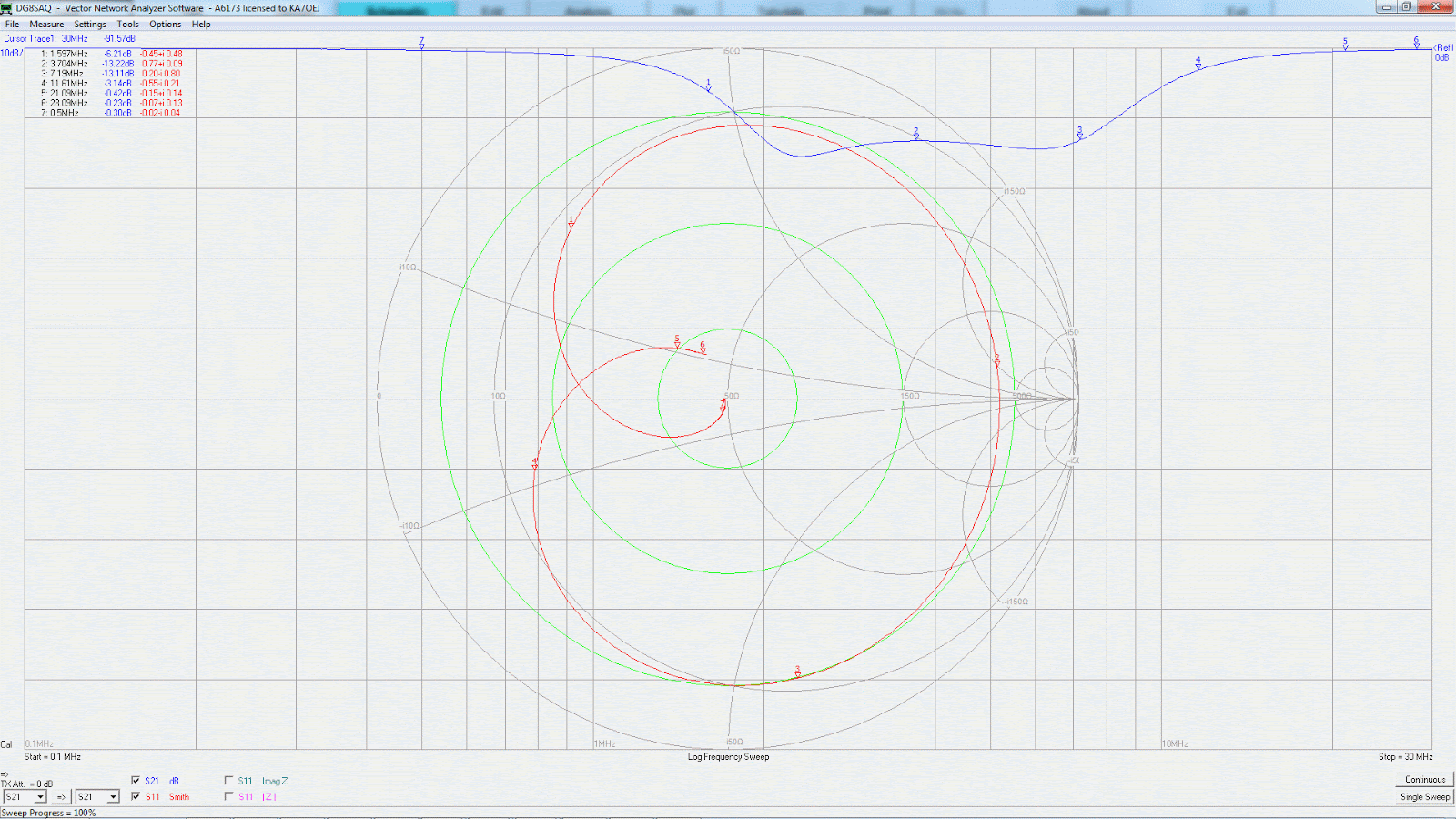
The response plot of the limited-attenuation band-stop filter.
Its effect is limited from the top end of the AM broadcast band and down, having at least 10dB of attenuation from about 1.8 MHz and 8 MHz with 13-15dB being more typical between these frequencies.
Click on the image for a larger version

The schematic of this device of may be seen here:

Figure 3:
Diagram of the limited-attenuation band-stop filter.
Click on the image for a slightly larger version.

If you have visited the 15 February, 2018 page, you will notice very distinct similarities between its main filter element and this circuit, right down to the application of signal "bypass" to set a maximum amount of attenuation that can occur.

In this filter, L1/C1, L2/C2 and L3/C3 are resonated to 3.7 MHz with the values selected to provide the desired attenuation at the frequencies at which the cut-off is to begin.  In this case, this filter is a slightly-tweaked version of a 3-pole Butterworth filter designed for a 50 ohm termination and has a theoretical 3dB passband of 11 MHz centered at 3.7 MHz.  The theoretical -6dB points of basic filter - ignoring R1/R2/L4 - is approximately 1.6 and 8.5 MHz with the -1dB points occurring at around 1.1 and 11.8 MHz.

Components R1/R2/L4 provide a degree of "bypassing" that leaks a controlled amount of signal around this filter:  Without these components, the attenuation could be in excess of 60dB near 3.7 MHz, but as can be seen, the actual attenuation is around 14dB, +/- 1dB or so.  While a simple resistor could have been used to accomplish this, the L4 slightly reduces the attenuation at the high end of the HF spectrum while R2 suppresses some of the asymmetry seen in the bottom of the attenuation curve that is caused by L4.

Figure 4:
As-built limited-attenuation band-stop filter.  This circuit - later put in an enclosure - is built "Manhattan" style using a combination of molded and toroidal chokes.  The BNC connectors visible were temporary, used only on the workbench for testing and characterization.  L1 and L2 are the black devices about the center, L2 is the red toroid in the foreground and L4 is the molded choke located close to the center pin of the right-hand BNC connector.
Click on the image for a larger version.

Comments:

• As can be seen from the Smith chart in Figure 2, this filter provides a 50 ohm match only at frequencies removed from the portion where the attenuation is occurring.  For this reason it is recommended that this filter be placed fairly close to the receiver (or splitter, if several receivers are being used) - this, to prevent impedance transformation on the line.  Similarly, it is recommended that this filter be preceded one stage of amplification to source the filter with something near-ish 50 ohms.
• If amplification is used for the receiver, it is suggested that the bulk of amplification be placed immediately after this filter:  The attenuation at the lower frequencies will reduce the probability of amplifier overloaded by the often-strong signals at these frequencies as well as the summer static.  The impact of the filter on the system noise figure at low frequencies is offset by the typically-high noise level while the low loss of the filter at higher frequencies which means that there will be little overall impact at the high end of the HF spectrum.
• In the case of the KiwiSDR system at the Northern Utah WebSDR, the total amount of amplification is about 22 dB in two stages:  At least 10dB is required in the overall system just to bring the receiver's noise floor (at 30 MHz) below the "rural quiet" noise floor - and there are likely to be other system losses that require even more amplification.  At the Northern Utah WebSDR, there is about 5 dB of loss between the antenna and the first amplifier, and there is an additional 6.5-7dB of loss in a four-way splitter to feed all of the receivers, so the overall 22dB gain in the system is about right.

This page stolen from ka7oei.blogspot.com

[End]