The Comcraft CTR-144 FM transceiver - A "multi-mode" solid state 2 Meter transceiver from the early 1970s.

Comcraft
Logo

Back in 1972 an ad appeared in the Ham magazines for something that probably seemed amazing at the time:  A solid state transceiver that covered the entire 2 meter amateur band (144-148 MHz - plus adjacent MARS and CAP frequencies) and did not need crystals!  This was the Comcraft CTR-144.  This radio cost $389.95 according to an advertisement in the January, 1972 issue of 73 magazine and was later listed at $489.95 in an ad in a 1973 73 Magazine advertisement (see Figure 6):  These prices are equivalent to over $3000 in 2026 dollars - for a two meter transceiver!

About Comcraft

Figure 1:
The Comcraft CTR-144 - a VFO solid-state 2 meter
FM/AM transceiver from the early 1970s.  A ham today
would probably be at loss when trying to use it!
The large knob is for tuning the receiver while the "VFO
Tuning" is for the transmitter frequency.  Aside from the
"tune" and "load" controls the rest are self-explanatory.
Click on the image for a larger version.

I haven't been able to find much about the Comcraft Company, other than it was in Goleta, California and that it seemed to exist from at at least 1971 until some time after 1976 when they released one of the earliest synthesized 2 meter transceivers, the CST-50.  I suspect that they may have made products for other markets, but I haven't been able find additional information.

More about the CTR-144

The CTR-144 is a "multi-mode" 2 meter transceiver in the sense that it can operate using both FM and AM - the latter being still present on the band in the early 1970s, but on its way out of common usage.  Compared to radios made since, this is an "odd duck" in the sense that it has separate tuning for the receiver and transmitter, both using VFOs - although it can accommodate three internal and one front-panel crystal for transmit for frequently-used repeaters and those applications that required good frequency stability and accuracy (e.g. MARS, CAP).  In other words, it doesn't have a conventional switch for a +/- 600 kHz repeater offset like that of modern radios, but rather you have to tune the transmitter and receiver separately to the repeater's input and output frequencies, respectively.  Additionally, it has a built-in power supply which allows it to operate from 120 Volts AC as well as a 12 volt input and provisions for a battery pack for "portable" use.

Figure 2:
The power amplifier section of the CTR-144 - solid-state
from the early 70s.  The "tune" and "load" air-variable
capacitors are visible, as is the side-mounted antenna jack.
Click on the image for a larger version.

As with some other radios recently featured on this blog, I acquired this one from a silent key friend of mine - and even into the early 2020s, he'd occasionally use this transceiver on some of the local repeaters that didn't require a subaudible tone.  It also has a very wide range "S-meter" which, unlike meters on most modern FM transceivers, would give a repeatable, reliable indication of signal strength over a range of just a microvolt or so to extremely strong. ¹  Being able to operate from a 12 volt vehicle and combined with the S-meter's wide dynamic range also made it a decent receiver for direction-finding not only with a small directional antenna, but to know when one was getting very close to the transmitter itself.

About the transmitter

The transmitter isn't particularly high-power:  The specifications state that it's rated for 12 watts input power with about 6 watts out. ² Considering the efficiency of early 1970s VHF power transistors, the output power of this transceiver is still in the range of 4-6 watts across the band, depending on frequency and supply voltage - plenty of power for local and moderate-distance repeaters when used with a modest outdoor antenna.

Figure 3:
Harmonic measurement of the Comcraft CTR-144.
Before the mid-late 70s there were no specific FCC rules
for the spectral purity of VHF transmitters, but current rules
still allow transmitters of that vintage to be used despite this.
Were it made today, the CTR-144 would not pass muster.
Click on the image for a larger version.

Out of curiosity I checked this transceiver's spectral purity on my service monitor (see Figure 3) and I wasn't terribly surprised at what I found:  While there were a few minor non-harmonic spurious emissions that were at least 40dB down from the carrier, the second harmonic was around -27 dBc - roughly 4 milliwatts.  While this would not be given a "pass" if the radio was made today (the current rules state that spurious/harmonic signals of a transmitter with 25 watts or less should be -40 dBc) there were no such rules prior to about 1977.  As noted in the current FCC rules, (§97.307(e)) a radio from this era is exempt from these rules but, if using a radio such as this causes interference, the onus is still on the amateur to resolve any issues.

If one looks at Figure 1 you'll see that there are two tuning knobs:  The larger one labeled "Tuning" - which is coupled to the slide rule that covers 144-148 MHz - is for the receiver, but the smaller one, labeled "VFO Tuning" is what sets the frequency of the transmitter and it is completely independent of the receive frequency.  What this means is that if you wish to use a repeater, the receiver is tuned to its output and the transmitter is set to its input frequency which, in the day, may have been a bit of a challenge:  The VFO Tuning (for transmit) knob doesn't have a great deal of tuning resolution on its dial so getting it "on frequency" back in the day probably meant setting the knob as close as possible visually and then getting "talked in" to the proper frequency.  When using this transceiver, my friend would have a frequency counter handy to allow him to dial in the transmit frequency precisely and monitor it for drift.

The transmit VFO itself operates from 7 to 9 MHz and this frequency is then mixed with a 65 MHz crystal to yield 72-74 MHz - and this is then doubled to the 144-148 MHz 2 Meter band.  With this scheme the transmit frequency could be reasonably stable as the most drift-prone component, the 6-9 MHz VFO, was operating at a low frequency.

A close inspection of  the front panel  in Figure 1 will reveal - along the right edge of the front panel - both a "Tune" and "Load" control.  For anyone using a radio with vacuum tube finals, controls labeled thusly would be familiar, but as this transceiver has a solid state amplifier these simply provide peaking/matching for final amplifier as indicated on the "S" meter rather than the "dip and load" of the older technology.

Figure 4:
The bottom of the CTR-144 showing the
rather hefty power transformer and, on top,
the doubler stage for the transmit chain.
The modulation transformer can be seen to
the left of the large, blue capacitor.
Click on the image for a larger version.

To produce frequency modulation it is the 7-9 MHz VFO itself that is modulated, but if a crystal is used, phase ³ modulation is applied to its oscillator's output prior to being multiplied by 18 to the desired transmit frequency.  For AM, high-level modulation is accomplished by using an audio amplifier to modulate the +12 volt supply for both the final amplifier transistor and its driver via the windings of an autotransformer - a rather "old school" way of doing it, but one that eliminates the need for another, higher-voltage power supply to achieve the desired peak output power. ⁴

About the receiver

While schemes to up-convert a low-frequency VFO for transmitting had been used for a long time, the way this transceiver goes about receiving is a bit more interesting and complex.  While more modern analog receivers would generate a local oscillator near the receive frequency and convert the desired signal to one or more lower-frequency IF (Intermediate Frequency) stages where a single channel would get demodulated, this works more like the receive section of a transverter in that the entire 2 meter band is is down-converted to the range of 14-18 MHz using "high-side" injection (e.g. the local oscillator is above the receive frequency) at 130 MHz from the same 65 MHz crystal as is used for transmit.

The receive VFO - the one tuned by the large knob with the frequency indicated by the slide rule - tunes across the 14-18 MHz IF to down-convert the received signal down to a fixed IF of 2 MHz where it is filtered and demodulated by a CA3075 integrated circuit.  The receiver front end itself uses some MOSFETs for amplification and mixing - a technique still used on superheterodyne receivers made today - and its sensitivity is as good as any receiver made today.

Using the CTR-144 on the air today

Figure 5:
The front end and receive section of the CTR-144.
The three-section air-variable capacitor tunes the local
that down-converts from the 14-18 MHz first IF to the 2 MHz
second IF where an integrated circuit is used for audio
demodulation.  In the upper-left is the MOSFET front-end
and filtering that give this radio good sensitivity - even by
today's standards.
Click on the image for a larger version.

Using the CTR-144 today is admittedly awkward compared to a modern radio, even if that the lack of subaudible tone for transmit wasn't an issue.  The receiver's slide-rule dial will get you "pretty close" to frequency, but unless the signal is actually present, you won't be able to tune it in for certain.  For simplex use, once you have tuned the receiver, there is a "Spot" switch that will inject a weak signal into the receiver that you can use to tune the transmit VFO to the same frequency by listening for and zero-beating it:  In this way the transmit and receive frequencies will be very close to each other.

Repeater operation is another matter. ⁵  Back in the 1970s you might have spent a few dollars to get transmit crystals for your favorite repeaters which would circumvent the problem of not knowing one's exact transmit frequency with the VFO.  But what if you didn't have a transmit crystal for the frequency?  Here, the "Spot" button is less-useful since, unless you happen to tune in someone's signal as they are transmitting to the repeater on its input frequency, there would normally be no signal at all to which you could precisely set its frequency.  While my friend, in later years, had a frequency counter in his ham shack so that he could determine precisely the transmit frequency, such a luxury that would have been unthinkable when this radio was first introduced. ⁶

Figure 6:
A Comcraft advertisement from
the April, 1973 issue of
73 Magazine
Click on it for a larger version.

Final comments

• When I first placed this transceiver on my workbench, it worked perfectly (although I haven't tried the built-in AC power supply) aside from two of the #47 dial lamps having burnt out.
• When the sensitivity was checked, it was only slightly deaf, but just a couple of minutes of time with the service monitor and tweaking the RF and IF stages brought it into specs.  It's interesting that while the manual (see link, below) has some "adjustment" information, it doesn't have a fully-detailed alignment procedure for the transceiver, likely because, as is true today, few people would have access to the necessary equipment to accomplish the task.  As it was, the manual and schematic informed me as to how it worked I was able to come up with a procedure "on the fly" to bring the radio back up to snuff.
  
• When 2 Meter FM first appeared, the amateur community had not yet standardized on what we now call "Wide" FM (e.g. +/-5 kHz deviation).  Different channel spacings and modulation widths could be found in different parts of the country, including +/- 15 kHz deviation - particularly on UHF.  The manual for the CTR-144 specifies a deviation of +/-7.5 kHz - yet another "standard"!
• The specified receiver bandwidth is 22 kHz which is somewhat wider than the typical 15-17 kHz for a "wide" FM receiver intended for +/-5 kHz deviation.  With this bandwidth - plus the probability of the receiver's tuned VHF frequency not being centered and an adjacent-channel repeater (15 or 20 kHz away, depending on the spacing in your area) - its use is likely to result in received interference.

Comcraft CTR-144 manual

I was fortunate enough to find the manual for this transceiver in my friend's files which has been scanned and may be found at this link:  Comcraft CTR-144 Manual (35 MB, .PDF).  At the time that this blog was posted, this manual was not to be found anywhere else on the Internet.

* * * * *

Footnotes:

1. On most FM transceivers, the S-meter will start indicating on very weak (and possibly noisy) signals and hit the "peg" (e.g. full-scale) even on a signal that is only modestly strong.  What this means is that for direction-finding purposes, most modern FM transceivers will give a "pegged" S-meter indicating even if you are some distance from the transmitter.  The CTR-144 on the other hand reaches full scale only if you happened to be right next to the transmitter while at the same time it starts indicating on a signal that is almost too weak to copy meaning that it could be used both at a great distance or in the final search for an unknown transmitter. 
2. Until the mid-late 1970s, amateur radio power limits were specified as input power to the final amplifier stage.  This method of transmitter power was likely an artifact of the days before RF power meters were common:  It's trivial to calculate the input power to the final amplifier if one knows the current and voltage, but that isn't the case for trying to measure RF power.
3. "Phase" modulation doesn't change the frequency directly but rather it "wiggles" the phase of the signal in accordance to the applied audio whereas actual "Frequency" modulation does change the frequency of the signal - in this case, by electrically shifting the VFO frequency:  Mathematically, the two are related since, if you could continually change the phase, frequency modulation would be the result.  With "FM" as used in the amateur service, one need only be able to modulate down to 200 Hz or so for voice meaning that with phase modulation, you could "temporarily" change the phase enough to effect a temporary de-facto frequency shift.  As the amount of change from a single phase modulator stage is quite small (perhaps +/- 60 degrees) this is usually applied at a lower frequency - in this case, at the 8 MHz crystal frequency and since this is multiplied by a factor of eighteen, our original +/-60 degrees of phase change becomes (18 * 60) 1080 degrees which is enough to appear as an adequately-modulated "FM" signal.  Mathematically, if one boosts the "highs" of the audio at a rate of 6dB per octave (e.g. doubling the deviation with every doubling of frequency) a signal generated using "FM" is indistinguishable from one that was originally phase modulated.  In fact, it is "PM" (Phase Modulation) that we use on "FM" as amateurs:  The "highs" in the audio are boosted (e.g. "emphasized") on transmit as they are the first to get noisy with a weak signal, and on receive they are restored back to their original level (e.g. "de-emphasized") which effectively reduces the amount of noise that is heard and makes weak, noisy signals more "listenable".
   
4. "High-level" modulation typically refers to applying the audio to the output RF stages(s) of a transmitter by increasing/decreasing the supply voltage.  Traditionally, this was done with an audio amplifier driving modulation transformer:  On peaks with 100% modulation the voltage applied to the final amplifier is approximately doubled, yielding the  four times the peak envelope power - but it also allowed the voltage to go to near zero at the other extreme.  On this transceiver, an audio amplifier drives an auto transformer (e.g. one with a single, tapped winding).  With no modulation, the 12 volt power supply for the finals goes through it unchanged, but with audio, the transformer action allows the requisite 24-volt(ish) peaks to be applied to the amplifier stage - all without needing the complexity of a 24 volt power source.  This method was "old" even when this radio was made, but it is simple and effective.
5. When this transceiver was made it was fairly rare for an amateur repeater to use a subaudible tone as doing so would mean that an amateur using it would not only have to have the proper crystals (for most radios of the day) but also a means to produce the needed subaudible tone frequency,  Later, in some areas subaudible tones were introduced when a geographically-adjacent repeater was on the same frequency to prevent users in an overlap area from bringing up both repeaters.  In some cases in amateur radio service, subaudible tones are used owing to occasional interference issues:  This is often considered to be a "band-aid" solution to a problem that is often due to the repeater's receive signal path not being able to adequately reject off-frequency signals (e.g. overload) - but sometimes it might be needed on a "busy" site where other users' gear isn't as well-filtered as it should be.
6. Back in the early 1970s a frequency counter of any sort would be a somewhat rare and expensive piece of test equipment - and this would be particularly true for one that could operate at VHF!  By the late 1970s and early 1980s technology had progressed to the point where such devices were more affordable and available to the average amateur. 

 * * * * *

This page stolen from ka7oei.blogspot.com 

 

[END] 

Adding FM transmit to the mcHF transceiver

In previous postings I wrote about how FM reception - including squelch and subaudible tone detection - was accomplished on the mcHF.  As is often the case, it is usually more difficult to receive a signal than to generate one and this is arguably the case with FM as well.

In writing the code to generate FM I found the above to be true:  It was comparatively trivial to produce an FM signal, particularly applying "tricks" that I'd already done in the demodulation.

Producing the FM carrier:

One of the features that I added to the mcHF many code releases back was that of "Frequency Translation" in which the local oscillator was "off-tuned" from the receive frequency, + or - 6 kHz for the mcHF with the "baseband" signals for receive and transmit being shifted by 6 kHz (in the opposite direction) in software.

One reason that this was done was to improve the performance of the transceiver by removing its receive and transmit passbands from the immediate vicinity of the "zero Hertz hole" which not only improves frequency response, but it reduces other issues related to thinks like "1/F" noise and, perhaps most importantly, greatly reduces the likelihood that other receiver audio (e.g. audio amplifier energy) will find its way back into the microvolt-level audio paths via power supply and ground loops and cause feedback!

Applying this to transmit, we soon realize that if wished to produce a signal with a constant carrier, such as AM or FM, we would have to remove ourselves from this "zero Hertz hole" as it would be, by definition, impossible to produce a carrier in that hole as a the carrier is, in fact, represented by DC.  (For SSB, which purposely has its carrier removed, this "hole" is nearly irrelevant...)

This explains another reason why this feature was added:  The eventual addition of AM transmission (and reception) several revisions ago, but this same feature used once again for FM, but in a different way:  Via the use of DDS (Direct Digital Synthesis) techniques.

The use of DDS techniques has been discussed on this blog before - see the article "Generating low-distortion audio sine waves using a PIC and DDS techniques." - link.

Using DDS techniques to generate an FM carrier:

In this technique one generates a sine wave (or any other arbitrary signal, for that matter) by jumping through a "lookup table".  In the case of the mcHF, with its 48 kHz sample rate, if we wanted to generate a 6 kHz sine wave this implies that we would need to step through this sine wave table once every 8 samples.  This sounds easy enough - but how would one do this?

Take a look at this bit of code:

loop:
   accumulator = accumulator + frequency_word
   table_index = accumulator > (size of accumulator in bits - size of table index in bits)
   amplitude = sine_table[table_index]

To explain the above:

- The variables "accumulator" and "frequency_word" are both integers.  Let us presume 16 bits, unsigned, each, which means that each value would range from 0-65535.  Incremented past 65535, it would return to zero.
- "sine table" is a lookup table containing values mapped to a sine wave.  Let us presume that our sine table contains 1024 entries - a number that may be represented by precisely 10 bits.
- "table_index" is used to index the table.  It must be able to index all of the sine table (10 bits) so we will use a 16 bit value for this.
- "amplitude" is the result from the sine table.  This could be an integer or floating point value - whatever format your system ultimately requires.

To calculate the value of "table index" we need to take the top 10 bits of the "accumulator", which means that we can obtain by taking the accumulator value and shifting it to the right by 6 bits (e.g. size of accumulator in bits, minus the size of table index in bits, which are 16 and 10, respectively.)  By doing this we can see that as the value of "accumulator" increases, it also points farther along the sine table.  When the value of accumulator "rolls over" back to zero, the pointer into the sine table also resets back to the beginning.

To understand how the frequency is generated, let us now assume that "frequency word" is set to 1.  We can see that every 65536 times through the loop we will "roll" through an entire sine wave, but since our sample rate is 48 kHz, we know that the produced frequency will be:

48000 / 65536 = 0.732 Hz (approx.)

If we want to generate an arbitrary frequency, we would take the above ratio and use it to calculate the "frequency word" as in:

desired frequency / (48000/65536)

or, rewriting a bit:

(desired frequency * 65536) / 48000

or, reducing the fraction even more:

(desired frequency * 512) / 375

If we wanted to generate a frequency of precisely 6 kHz, the above equation would yield a "frequency word" value of 8192 - which just happens to be exactly 1/8^th of 65536, which makes sense since we have already figured out that since 6 kHz is 1/8^th of our sample rate of 48 kHz, it would therefore take 8 samples to produce such a sine wave!

Modulating our carrier:

We now know how to generate a carrier, but how to modulate it?

We know that FM is simply "Frequency Modulation", and we also know that by varying the value of "frequency_word" above, we can change the frequency, does this mean that if we superimpose audio on our value of "frequency_word" that we can modulate our signal?

Yes, it does.

Let us rewrite the above code a bit:

loop:
   accumulator = accumulator + frequency_word + audio[audio_index++]
   table_index = accumulator > (size of accumulator in bits - size of table index in bits)
   amplitude_I = sine_table[table_index]
   table_index = table_index + 256
   if(table_index >= 1024)
      table_index = table_index - 1024
   amplitude_Q = sine_table[table_index]

(Let us assume that "audio_index" is updated each time through the loop and represents one sample of the audio, also sampled at 48 kHz, to be modulated onto the carrier.)

Let us first take a look at the first line after the start of the loop where we added the term "audio".  Because our audio is already represented digitally as a numerical value that goes above zero for a positive voltage and below zero for a negative voltage, it would make sense that we could simply add this to our "frequency_word" value.

In other words (pun intended!) when the audio voltage increased above zero, our frequency would increase, but as it went below zero, our frequency would decrease - just as FM would.  What's more, because this is an exact numerical representation, our frequency change would be proportional to the audio applied - which is just want we want to occur for low-distortion, faithful representations of our audio.

Figure 1:
A demonstration of a typical FM signal modulated with a tone as
displayed on the mcHF's waterfall display.
(This picture doesn't have much to do with transmitting, but
I wanted to include some color in this posting!) 

There is another modification to the above code as well.  If you look, you will see that we do two look-ups in the "sine_table".  The first one is our original value, now called "amplitude_I" (In-phase) but we now see that we have taken our table index and added 256 to it which is precisely 1/4^th the size of our sine table:  One quarter of a sine wave is, of course, represented by 90 degrees.  After "fixing" that value so that it is always lower than 1024, we look up into the sine table again and call this value "amplitude_Q".

What we have done here is generated two sine waves exactly 90 degrees apart from the same frequency synthesis operation.  As you will recall from your understanding of the "phasing" required to generate an SSB signal, you need both an "I" and "Q" signal for transmit and unlike the generation of quadrature audio for SSB which requires some fairly "hairy" math, we have handily done this for FM with almost no math at all!

Comment:  In reality one would employ modulus operators rather than "greater-than and subtract" or even logically "AND" the table index value with 1023 (decimal) after adding 256 to it, either being a much quicker operation for a computer than in the example shown above.

Additional audio processing:

As was mentioned in the discussion about the demodulator, for amateur radio purposes we don't actually want to transmit an "FM" signal, but really a "PM" (Phase Modulated) signal.  For our purposes, a PM signal is really an FM signal in which the audio is pre-emphasized at a rate of 6dB per octave - which is a fancy way of saying that a signal voltage that causes +/- 1 kHz of deviation with a modulation frequency of 1 kHz would cause +/- 2 kHz of deviation with a modulation frequency of 2 kHz.  As noted in previous postings, this is done to improve the overall signal-noise performance of the system as it boosts the "highs" in the audio at about the same rate as the noise increases on weak signals.

There are some practical issues with this pre-emphasis that must be considered.  If you were to start your pre-emphasis at 1 Hz, by the time you get to 2048 Hz would have pre-emphasized your audio by 66 dB or so (if I've done my math right) - a ridiculous amount, and any audio content that might be present at higher frequencies would be boosted even more!  Such high frequency content would also cause high amounts of deviation which, in turn, would greatly expand the occupied bandwidth of the transmitted signal - something that is neither necessary or neighborly!

Clearly, this implies that we must do two things:

• Limit the frequency range over which we do our pre-emphasis
• Filter the the audio to the desired range for speech communications

If we start our pre-emphasis at around 200 Hz, instead, we can see that by the time we get to 3200 Hz we need to boost only by 36 dB - a far more reasonable value than the 66 dB mentioned above!

For speech we need only reproduce audio from around 250 Hz to something in the area of 2500-2700 Hz.  Our low-frequency limit is imposed by our desire to include the encoding of "subaudible" tones on our transmitted signal and it is important that we remove a reasonable amount of energy in that frequency range so that spectral content of the human voice - particularly that of the adult male - does not encroach in that area and cause reliability problems with decoding on the receiving end.

Fortunately, such tools are already at hand!

Pre-emphasis:

We already met the differentiator algorithm in our receiver as it was used to reduce the low-frequency, subaudible tones from received audio.  This algorithm reproduced below.

loop:

  filtered = α * (old_input + input - old_filtered)

  old_filtered = filtered

  old_input = input

Where:
  "α" is the the equivalent of the time constant in that a "small" α implies an R/C circuit with a fast time-constant strongly affecting "low" frequencies.
  "input" is the new audio sample.
  "filtered" is the high-pass filtered (differentiated) audio

In the case of the receiver we used it as a high-pass filter with a cut-off below the speech range, but for transmit we can adjust the "knee" of this differentiator such that it is just above the speech range, instead.  As it turns out, an "α" value of 0.05 is suitable for our purposes.

Filtering:

Having done pre-emphasis, we still need to do filtering, but I'd already implemented a "transmit" filter on the mcHF for both SSB and AM and all I needed to do was redesign the filter to suit the FM audio characteristics.  I used MatLab and the filter designing plug in for this, but the "Iowa Hills" filter designer suite (free and easily found via a web search) could be used to produce suitable sets of coefficients.  As are most of the filters used on the mcHF, these filters were IIR since one can get a lot of "bang for the buck" in terms of good, "sharp" filtering with relatively few computation cycles.

With a fairly compact filter with fairly low computational overhead I was able to achieve >20dB of voice rejection in the upper frequencies used for subaudible tones and well over 50 dB of attenuation above 3200 Hz - much better than that achieved in a typical, analog FM transmitter.  At the low end, audio below 250 Hz was attenuated by at least 20dB with over 40 dB reduction for audio content below 200 Hz - this, to prevent "pollution" of the frequencies occupied by subaudible tones.

Comment:  Because I was using floating-point math, the order in which pre-emphasis or filtering is done is unimportant.  If fixed-point/integer math was used, instead, you would need to carefully analyze the signal path and the resulting values to assure that nothing "blew up" (e.g. exceeded the integer range or, at the other extreme, was so "small" that resolution was compromised and distortion/noise introduced) at the expected audio levels at all frequencies!

Limiting:

One necessary function employed in typical amateur FM transmitters is that of the limiter to "clip" the audio to an absolute maximum level.  This device improves overall intelligibility by allowing the designer to set the microphone gain to a somewhat excessive level, but the clipper forcing a maximum loudness.  The result of this is that somewhat low audio from soft-spoken users is boosted to promote intelligibility while those who have "hot" microphones and/or speak loudly do not cause excess amounts of deviation of the transmitted signal.

The mcHF does not have a clipper, per se, but it does have an audio compressor that was implemented many versions ago to improve usability on SSB.  Like a limiter, this device prevents the audio from exceeding an absolute maximum level and it also adjusts the gain upwards during quiet portions to reduce the "peak-to-average" ratio of the audio, thereby improving intelligibility.

I did experiment with both a "hard" and a "soft" limiter (or clipper) in software.  A "hard" limiter is one that sets an absolute ceiling on the amplitude of the signal present while a "soft" limiter, as the name implies, is less abrupt, more like the "knee" of a diode with some sort of logarithmic-like action.  Because they alter the waveforms, both of these methods generate harmonics and intermodulation products - the "soft" limiter being a bit less aggressive - which require that filtering be done.  Since we are low-pass filtering the audio, the higher-frequency harmonics outside the speech range will not contribute to the occupied bandwidth of the signal but the increased energy in the upper speech frequencies from harmonics of the lower-frequency audio components coupled with the pre-emphasis can somewhat broaden the signal.  Finally, because the signal is distorted by the clipping action, high audio levels that result in a lot of clipping are likely to result in audio that "sounds" degraded.

In comparing the sounds of the limiter/clipper to that of the audio compressor, I decided to use the latter as it was more "pleasing" to the ear and more versatile, overall since there are a number of available adjustments (e.g. the amount of audio into the variable gain stage and the decay rate of the variable gain stage.) As noted, I eventually decided not to use a clipper and used the already-existing compressor, instead.

Without either this compressor or a limiter, an FM transmitter would have the problem of their signal being "too wide" for loud-speaking operators and "too quiet" for those that were soft spoken - neither condition being desirable for communications!

Subaudible tone:

A desirable feature of a modern FM transmitter is that of the Subaudible Tone, discussed previously.  This signalling method consists of the generation of a low-level sine wave in the range of approximately 67 to 250 Hz that is superimposed on the transmitted audio which is used by the receiver to validate the presence of signal.  While this was traditionally used in commercial radio to allow several groups of users to "share" the same frequency, amateurs have typically used it as interference mitigation techniques to prevent the receiver - that of the repeater or the user - from responding to noise or signals for other sources.

For additional information about subaudible tone signalling, read the Wikipedia article - link.

Since it is just a sine wave, it is very easy to generate - and we already know how!

Re-using the DDS algorithm, above, we need only generate a single tone, unmodulated this time, and sum it with our transmitted audio.  We would of course, do this after we have done our pre-emphasis, filtering and limiting/compressing, placing this tone generator just before the DDS that produced our FM signal as the code snippet below illustrates.


[Filtering and limiting/clipping of audio already done]

if(tone_generator=TRUE) {
      tone_accumulator = accumulator + tone_frequency_word
      table_index = tone_accumulator > (size of tone accumulator in bits - size of table index in bits)
      tone = sine_table[table_index]
      audio = audio + (tone * amplitude)
}

[The code that follows is the DDS that generates the FM signal as shown above]

As we can see, only if the tone generator is turned on do we go through the loop - something that we'd do to save processing power.  Included in the above code snipped is an additional parameter, "amplitude" which would be used to scale the value from the sine lookup table such that it yielded the proper amount of deviation on the transmitted signal - typically in the area of 15-20% of peak deviation.

In the case of generating the audio tone we'd need to make certain that we had enough frequency resolution to accurately produce the tone, and as we already calculated we know that with a 16 bit counter at a 48 kHz sample rate our resolution is approximately 0.732 Hz. Assuming no sample rate errors, this would imply that we could generate the desired frequency to within half that resolution worst-case, or approximately 0.366 Hz.

This frequency resolution is adequate for generation of these tones, again assuming that there are no additional error sources related to sample rate, but if you were not satisfied with that amount of resolution it would be a fairly simple matter to increase the number of bits used by the accumulator and frequency word to improve the resolution, just as was suggested for the frequency modulation.

For the calculation of the frequency words, all that was required was that the code include a table containing the frequency, in Hertz, of each of the subaudible tones:  Since we already know the sample rate and the number of bits - and therefore the maximum counts for our accumulator - we can calculate, on the fly, the needed "frequency word".

Tone burst:

There is one more tone signalling scheme occasionally encountered on FM repeater systems, and that is the "tone burst", sometimes called "Whistle-up".  Although it has largely disappeared from use, it is reportedly used in some areas in Europe.

In this system a short burst of a specific tone, typically 1750 or 2135 Hz, is transmitted to "wake up" a repeater for use, and once this is done, it may be used normally.  Once the repeater has again become dormant, a timer expires and it will no longer respond to signals until it, again, receives a burst.

For a Wikipedia article that includes a section about single-tone signalling, look here:  link

This is generated in exactly the same way as a subaudible tone, namely with a bit of DDS code that looks just like the above!  From a purely practical standpoint, unless one absolutely needed to generate both a subaudible tone and a tone burst at the same time, one could actually use the same bit of code - provided that the amplitudes of the different tones (subaudible, burst) were taken into account.

Unlike a subaudible tone, a tone burst is typically transmitted only at the beginning of a transmission and for a fairly short period - perhaps one second.  While one could rely on the user to time the duration of the tone burst, on the mcHF the duration of the burst was timed by counting the number of interrupt cycles called to process the audio, making the process semi-automatic:  The user needed only activate push-to-talk and then press-and-hold the button that produced the tone and the rest would be completed automatically.

"DCS" codes:

Not mentioned previously there is one additional signalling scheme sometimes found on amateur frequencies, and that is "DCS" (Digital Coded Squelch) which consists of a binary signal with a base frequency of 134.4 Hz modulated with a specific bit pattern.  This signalling scheme is quite rare in the amateur radio community - and even rarer on HF (10 meter) repeaters where this radio is likely to be used - so there has been no serious consideration in its support


How well does it work?

Generating a sine wave with a low-distortion audio generator and feeding the modulated signal into a communications test set (a.k.a. "Service Monitor") - a device specially designed to analyze the quality of communications gear - the modulation was tested at several audio frequencies and found that the distortion was at approximately the level of detection of the instrument to at least +/- 5 kHz deviation.

Testing was also done using speech at various levels, including attempts to overdrive the audio input and on a spectrum analyzer the occupied bandwidth was observed to be contained within the expected bandwidth mask for both the "narrow" (+/- 2.5 kHz) and "wide" (+/- 5 kHz) deviation settings with no audible distortion present nor were there any unexpected spectral components outside the frequency range typical of such an FM signal - even though the "accumulator" of the frequency-modulating DDS is only 16 bits and the audio represented by it will have even lower resolution (e.g. on the order of 12 bits, maximum.)

At the present time I can't think of any additional features that would need to be added to the FM mode so it is, for now, "good to go."


[End]

This page stolen from "ka7oei.blogspot.com".

FM squelch and subaudible tone detection on the mcHF

In a previous installment  ("Adding FM to the mcHF SDR Transceiver" - link) I described how the demodulation of FM signals was added to the mcHF SDR transceiver but being able to receive FM implies the addition of a few other features, namely that of squelch "circuitry" - of both "carrier" and "tone" types.

Determining the "squelch" status of a received signal:

One of the most obvious ways to determine the presence of a signal is to compare the signal strength against a pre-set threshold:  If the signal is above that threshold it is considered to be "present" and an audio gate is opened so that it may be heard.

This sounds like a good way to do it - except that it isn't, really, at least not with FM signals.

If you were listening to an FM signal on 10 meters that was fading in and out (as it often does!) one would have to set the threshold just above that of the background noise - or "open" (e.g. disable) it completely to prevent it from disappearing when the signal strength dove into a minimum during QSB.  If the background noise were to vary - as it can over the course of a day and with propagation - the squelch would be prone to opening and closing as well.

As it turns out, typical FM squelch circuits do not operate on signal strength as there are better methods for determining the quality of the signal being received that can take advantage of the various properties of the FM signals themselves.

Making "Triangle Noise" useful:

Mentioned in the previous entry on this topic was "Triangle Noise", so-called by the way it is often represented graphically.

Figure 1:
A graph representing the relative amplitude of noise with strong weak FM signals.  It is the upward tilt of the noise energy to which "Triangle" noise refers - the angle getting "steeper" as the signal degrades.  Also represented is a high-pass filter that removes the modulated audio, leaving only the noise to be detected.
From this diagram one can begin to see why pre-emphasizing audio along a curve similar to the "weak signal noise" line can improve weak-signal intelligibility by boosting the high-frequency audio on transmit (and doing the inverse on receive) to compensate for the noise that encroaches on weak signals.

As can be seen in Figure 1 the noise in a recovered FM signal increases as the signal get weaker - but notice something else:  The noise increases more quickly at higher frequencies of audio than it does at lower audio frequencies.  Looking at Figure 1 you might make another observation:  Because there is typically some low-pass filtering of the transmitted audio to limit its occupied bandwidth, there is no actual (useful) audio content above that frequency from the distant station, but the noise is still there.

High-pass filtering to detect (only) "squelch noise":

From the above drawing in Figure 1 it can be recognized that if we only "listen" to the high-frequency audio energy that passes through the "Squelch noise" high-pass filter all we are going to detect is the noise level, independent of the modulated audio.  If we base our signal quality on the amount of noise that we detect at these high frequencies - which are typically above the typical hearing range (usually ultrasonic, above 10 kHz) - we can see that we don't need to know anything about the signal strength at all.

This method works owing to an important property of FM demodulators:  The amount of recovered audio does not change with the signal strength as the demodulator is "interested" only in the amount of frequency change, regardless of the actual amplitude.  What does change is the amount of noise in our signal as thermal noise starts to creep in, causing uncertainty in the demodulation.  In other words, we can gauge the quality of the signal by looking only at the amount of ultrasonic noise coming from our demodulator.

Figure 2: 
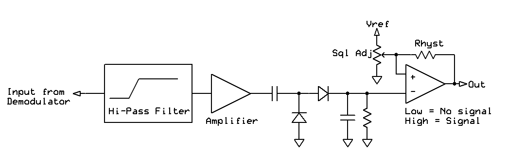
An representation of an analog squelch circuit with hysteresis.  The high-pass filter removes the "program" audio modulated onto the carrier (e.g. voice) which is then amplified as necessary and then rectified/filtered to DC to derive a voltage proportional to the amount of ultrasonic noise present:  The higher the voltage, the "weaker" and noisier the signal.
The resulting voltage is then fed with a comparator that includes hysteresis to prevent it from "flapping" when it is near the squelch threshold.

An analog representation of a squelch circuit may be seen in Figure 2.  For the simplest circuit, the high-pass filter could be as simple as an R/C differentiator followed by a single-transistor amplifier, and the same sorts of analogs (pun intended!) could be applied in software.

After getting the mcHF FM demodulator to be functional I tried several different high-pass filter methods - including a very simple differentiator algorithm such as that described in the previous posting - except, of course, that the "knee" frequency was shifted far upwards.  The absolute value was then taken from the output of the high-pass filtered and smoothed and printed on the screen while the input signal, modulated with a 1 kHz audio sine wave and fed to a SINAD meter (read about SINAD here - link) while signal level was varied:  In this way I could see how the output of the noise detection circuit behaved with differing signal conditions.

In doing this testing I noted that a simple differentiator did not work as well as I'd hoped - likely due to the fact that unlike an analog circuit in which the high-frequency energy can continue to increase in intensity with frequencies well into the 10's or 100's of kHz, in the digital domain we have a "hard" limit enforced by Nyquist, stopping at 23 kHz or so on the mcHF with its 48 ksps rate.

With less high frequency spectral noise energy (overall) to work with it is necessary to amplify the output of a simple differentiator more, but this also brings up the lower frequency (audio) components, causing it to be more affected by speech and other content, requiring a better filter.  Ultimately I determined that 6-pole IIR high-pass audio filter with a 15 kHz cut-off frequency, capable of reducing "speech" energy and its second and third harmonics below 9-10 kHz by 40-60dB, worked pretty well:  In testing I also tried a similar filter with an 8 kHz cut-off, but it was more-affected by voice modulation and its immediate harmonics.

Comment:

If the FM demodulation is working properly the result will be a low-distortion, faithful representation of the original audio source with little/no energy above the low-pass filter's cut-off in the transmitter.  If the signal is distorted in some way - such as with multipath distortion, being off-frequency or with excess deviation, energy from this distortion can appear in the ultrasonic region which cannot be easily distinguished from "squelch" noise.

If this energy is high enough, the squelch can close inadvertently since the signal may be "mistaken" as being weak:  This is referred to as "squelch clamping" and is so-called as it is often seen on voice peaks of signals degraded by multipath and/or off-frequency.

Determining noise energy:

In short, the algorithm to determine the squelch energy was as follows:

loop:

   squelch_avg = (1-α) * squelch_avg + sqrt(abs(hpf_audio)) * α
   if(squelch_avg > MAX_VALUE)
      squelch_avg = MAX_VALUE

Where:
   α = "smoothing" factor
   hpf_audio = audio samples that have been previously high-pass filtered to remove speech energy
   squelch_avg = the "smoothed" squelch output

If you look at the above pseudocode example you'll notice several things:

• The square root value of the absolute value of the high-pass noise energy is taken.  It was observed that as the signal got noisier, the noise amplitude climbed very quickly:  If we didn't "de-linearize" the squelch reading based on the noise energy - which already has a decidedly non-linear relationship to the signal level - we would find that the majority of our linear squelch adjustment was "smashed" toward one end of the range.  By taking the square root our value increases "less quickly" with noisier signals than it otherwise would.
• The value "squelch_avg" is integrated (low-pass filtered) to "smooth" it out - not surprising since it is a measurement of noise which, by its nature, is going to vary wildly - particularly since the instantaneous signal level can be anything from zero to peak values.  What we need is a (comparatively) long-term average.
• The "squelch_avg" value is capped at "MAX_VALUE".  If we did not do this the value of "squelch_avg" would get very high during periods of no signal (maximum noise) and take quite a while to come back down when a signal did appear, causing a rather sluggish response.  The magnitude of "MAX_VALUE" was determined empirically by observing "squelch_avg" with a rather noisy signal - the worst that would be reasonably expected to open a squelch.

Obtaining a usable basis of comparison:

The above "squelch_avg" value increases as the quieting of the received FM signal decreases which means that we must either invert this value or, if a higher "squelch" setting means that a better signal is required for opening the squelch, that same "squelch setting" variable must have its sense inverted as well.

I chose the former approach, with a few additional adjustments:

• The "squelch_avg" value was rescaled from its original range to approximately  24 representing no-signal conditions to 3 representing a full-quieting signal with modulation with hard limits imposed on this range (e.g. it is not allowed to exceed 24 or drop below 3).
• The above number was then "inverted" by subtracting it from 24, setting its range to 2 representing no signal to 22 for one that is full-quieting with modulation.

It is not enough to simply compare the derived "squelch_avg" number after scaling/inversion with the squelch setting, but rather a bit of hysteresis must also be employed or else the squelch is likely to "flap" about the threshold.  I chose a value of 10% of the maximum range, or a hysteresis range of +/-2 which seemed to be about right.

The final step was to make sure that if the squelch was set to zero that it was unconditionally open - this, to guarantee so that no matter what, some sort of signal could be heard without worrying about the noise threshold occasionally causing the squelch to close under certain conditions that might cause excess ultrasonic energy to be present.

The result is a squelch that seems to be reasonably fast in response to signals, weak or strong, but very slightly slower in response to weak signals.  This slight asymmetry is actually advantageous as it somewhat reduces the rate-of-change that might occur under weak-signal conditions (e.g. squelch-flapping) - particularly during "mobile flutter."  The only downside that is currently noted is that despite the "de-linearization" the squelch setting is still somewhat compressed with the highest settings being devoted to fairly "quiet" signals" and most of the range representing somewhat noisier signals - but in terms of intelligibility and usability, it "feels" pretty good.

Subaudible tone decoding:

One useful feature in an FM communications receiver is that of a subaudible tone (a.k.a. CTCSS) decoder.  For an article about this method of tone signalling, refer to the Wikipedia article here - link.

In short, this method of signalling uses a low-frequency tone, typically between 67 and 250 Hz, to indicate the presence of a signal and unless the receiver detects this tone on the received signal it is ignored.  In the commercial radio service this was typically used to allow several different users to share the same frequency but to avoid (always) having to listen to the others' conversations.  In amateur radio service it is often used as an interference mitigation technique:  The use of carrier squelch and subaudible tone greatly reduces the probability that the receiver's squelch will falsely open if no signal is present or, possibly, if the wrong signal - in the case where a listener is an an area of overlapping repeaters - is present - but this works only if there is a tone being modulated on the desired signal in the first place.

The Goertzel algorithm:

There are many ways to detect tones, but the method that I chose for the mcHF was the Goertzel algorithm.  Rather than explain exactly how this algorithm works I'll point the reader to the Wikipedia article on the subject here - link.  The use of the Goertzel algorithm has several distinct advantages:

• Its math-intensive parameters may be calculated before-hand rather than on the fly.
• It requires only simple addition/subtraction and one multiplication per iteration so it need only take a small amount of processor overhead.
• Its detection bandwidth is very scalable:  The more samples that are accumulated, the narrower it is - but also slower to respond.

The Goertzel algorithm, as typically implemented, is capable of "looking" at only one frequency at a time - unlike an FFT which looks at many - but since it is relatively "cheap" in terms of processing power (e.g. the most intensive number-crunching is done before-hand) it is possible that one could implement several of them and still use fewer resources than an FFT.

The Goertzel algorithm, like an FFT, will output a number that indicates the magnitude of the signal present at/about the detection frequency, but by itself this number is useless unless one has a basis of comparison.  One approach sometimes taken is to look at the total amount of audio energy, but this is only valid if it can be reasonably assured that no other content will be present such as voice or noise, which may be generally true when detecting DTMF, but this cannot be assured when detecting a subaudible tone in normal communications!

"Differential" Goertzel detection:

I chose to use a "differential" approach in which I set up three separate Goertzel detection algorithms:  One operating at the desired frequency, another operating at 5% below the desired frequency and the third operating at 4% above the desired frequency and processed the results as follows:

• Sum the amplitude results of the -5% Goertzel and +4% Goertzel detections.
• Divide the results of the sum, above, by two.
• Divide the amplitude results of the on-frequency Goertzel by the above sum.
• The result is a ratio, independent of amplitude, that indicates the amount of on-frequency energy.  In general, a ratio higher than "1" would indicate that "on-frequency" energy was present.

By having the two additional Goertzel detectors (above and below) frequency we accomplish several things at once:

• We obtain a "reference" amplitude that indicates how much energy there is that is not on the frequency of the desired tone as a basis of comparison.
• By measuring the amplitude of adjacent frequencies the frequency discrimination capability of the decoder is enhanced without requiring narrower detection bandwidth and the necessarily "slower" detection response that this would imply.

In the case of the last point, above, if we were looking for a 100 Hz tone and a 103 Hz tone was present, our 100 Hz decoder would "weakly-to-medium" detect the 103 Hz tone as well but the +4% decoder (at 104 Hz) would more strongly detect it, but since its value is averaged in the numerator it would reduce the ratiometric output and prevent detection.

Setting the Goertzel bandwidth:

One of the parameters not easily determined in reading about the Goertzel algorithm is that of the detection bandwidth.  This parameter is a bit tricky to discern without using a lot of math, but here is a "thought experiment" to understand the situation when it comes to being able to detect single-frequency (tone) energy using any method.

Considering that the sample rate for the FM decoder is 48 ksps and that the lowest subaudible tone frequency that we wish to detect is 67.0 Hz, we can see that at this sample rate it would take at least 717 samples to fully represent just one cycle at 67.0 Hz.  Logic dictates that we can't just use a single cycle of 67 Hz to reliably detect the presence of such a tone so we might need, say, 20 cycles of the 67 Hz tone just to "be sure" that it was really there and not just some noise at a nearby frequency that was "near" 67 Hz.  Judging by the very round numbers, above, we can see that if we had some sort of filter we might need around 15000 samples (at 48 ksps) in order to be able to filter this 67 Hz signal with semi-reasonable fidelity.

As it turns out, the Goertzel algorithm is somewhat similar.  Using the pre-calculated values for the detection frequency, one simply does a multiply and a few adds and subtractions of each of the incoming samples:  Too few samples (fewer than 717 in our example, above) and one does not have enough information with which to work at low frequencies to determine anything at all about our target frequency of 67 Hz, but with a few more samples one can start to detect on-frequency energy with greater resolution.  If you let the algorithm run for too many samples it will not only take much longer to obtain a reading, but the effective "detection bandwidth" becomes increasingly narrow.  The trick is, therefore, to let the Goertzel algorithm operate for just enough samples to get the desired resolution, but not so many that it will take too long to obtain a result!  In experimentation I determined that approximately 12500 samples were required to provide a tradeoff between adequately-narrow frequency resolution and reasonable response time.

This is part of the reason for the "differential" Goertzel energy detection in which we detect energy at, above and below the desired frequency:  This allows us to use a somewhat "sloppier" - but faster - tone detection algorithm while, at the same time, getting good frequency resolution and, most importantly, the needed amplitude reference to be able to get a useful ratiometric value that is independent of amplitude.

Debouncing the output:

While an output of greater than unity from our differential Goertzel detection generally indicates on-frequency energy, one must use a significantly higher value than that to reduce the probability of false detection.  At this point one can sort of treat the output of the tone detector as a sort of noisy pushbutton switch an apply a simple debouncing algorithm:

loop:

   if(goertzel_ratio >= threshold)   {
      debounce++
      if(debounce > debounce_maximum)
         debounce = debounce_maximum
   }
   else   {
      if(debounce > 0)
         debounce--
   }
   if(debounce >= detect_threshold)
      tone_detect = 1
   else
      tone_detect = 0

where:

   "goertzel_ratio" is the value "f/((a+b)/2))" described above where:
      f = the on-frequency Goertzel detection amplitude value
      a = the above-frequency Goertzel detection amplitude value
      b = the below-frequency Goertzel detection amplitude value
   "threshold" is the ratio value above which it is considered that tone detection is likely.  I found 1.75 to be a nice, "safe" number that reliably indicated on-frequency energy, even in the presence of significant noise.
   "detect_threshold" = the number of "debounce" hits that it will take to consider a tone to be valid.  I found 2 to be a reasonable number.
   "debounce_maximum" is the highest value that the debounce count should attain:  Too high and the it will take a long time to detect the loss of tone!  I used 5 for this which causes a slight amount of effective hysteresis and a faster "attack" than "decay" (e.g. loss of tone).

With the above algorithm - called approximately once every 12500 samples (e.g. just under 4 times per second with a 48ksps sample rate) - the detection is adequately fast and quite reliable, even with noisy signals.

Putting it all together:

Figure 3:
An FM signal with a subaudible tone being detected, indicated by
the "FM" indicator in red.

If tone decoding is not enabled, the Goertzel algorithms are not called at all (to save processor overhead) and the variable "tone_detect" is set to 1 all of the time.  For gating the audio a logical "AND" is used requiring that both the tone detect and squelch be true - unless the squelch setting is 0, in which case the audio is always enabled.

Finally, if the squelch is closed (audio is muted) the audio from the FM demodulator is "zeroed".


* * *

In a future posting I'll describe how the the modulation part of this feature was accomplished on the mcHF along with the pre-emphasis of audio, filtering and the generation of burst and subaudible tones.


[End]

This page stolen from "ka7oei.blogspot.com".

Adding FM to the mcHF SDR transceiver

This has been one of those "Rabbit Hole" features.

In the past I have stated several times on the Yahoo Group that I would not be adding FM to the mcHF (a completely stand-alone QRP SDR HF transceiver) any time soon, mostly because I was quite certain that there was simply not enough processor horsepower to do it properly, but quite recently I (sort of) got obsessed with making it work, going from "0 to 60" in just a few evenings of code "hacking".

While it took only an hour or so to get the FM demodulation and modulation working it ultimately took much longer than that to integrate the other features (subaudible tone encode/decode, etc.) and especially the GUI interface with everything!  By the time I was done I'd spent more time than I had hoped (not unexpected!) but at least had something to show for it!

FM on an HF transceiver:

First of all, FM is one of those modes that I have used on HF only a few dozen times in my 30+ years of being a ham - using it most often (albeit rarely) when 10 meters is open and I hear a repeater booming in, but other than that I haven't really had any reason to do so, particularly since there are no local 10 meter repeaters and local activity on "10 FM" is quite sparse.

Figure 1:
Reception of an FM signal as displayed on the waterfall (using the
"blue" palette) showing the sidebands from the 1 kHz tone
modulated onto the carrier being received.  The white background
on the "FM" indicator shows that the (noise) squelch is open.
Click on the image for a larger version.

What might be a practical reason to add FM to the mcHF other than for 10 meter openings or with a transverter (or a modified radio) on a higher band such as 6, 4 or 2 meters where FM is common?  I asked this question on the mcHF Yahoo group and several people noted that in various parts of Europe, FM repeaters and simplex operation on 10 meters is/are (apparently) more common than here in the U.S - not to mention the fact that I suspect that some mcHF users like to hang out on "CB" frequencies where FM is used in Europe.

Background:

As it turns out I was recently adding/fixing some of the current mcHF features, streamlining some code and I decided to look into what, exactly, it would take to demodulate FM.

Before I begin the description it should be noted that the mcHF, in FM receive mode, must utilize "frequency translation" which shifts the local oscillator by 6 kHz - this, to get away from the "0 Hz hole" intrinsic to many SDR implementations that down-convert the RF to baseband:  If we did not do this the FM carrier would land in this "hole" and hopelessly distort it!

With the signal to be received centered at 6 kHz at the input of the A/D converter, a software frequency conversion shifts it back to "0 Hz" where, in the digital domain, the hole does not exist.  True, the FM signal is now modulated +/- zero and includes "negative" frequencies, but since the signals are quadrature and it is just math at this point we can get away with it!

(Note:  The "0 Hz hole" still exists but is now 6 kHz removed from the center of the carrier so it has no effect at all on demodulated signals in receive bandwidths up to 12 kHz.)

The PLL method of demodulating FM:

The most common way to do this is via a PLL, implemented in software

Figure 2:  PLL implementation of an FM demodulator

Depicted in Figure 2 this works by "tracking" the variations of the input signal's frequency using the PLL:  Differences in instantaneous phase are detected, applied to the VCO's tuning line via the Loop Filter.  The loop filter is present to remove the energy from the original carrier frequency, effectively leaving only the audio modulation behind, a sample of which is high-pass filtered to remove the DC content and used to extract the demodulated audio.

In hardware this type of scheme is used in PLL ICs such as the NE564 and NE565, or even the good old 4046 PLL IC:  Many implementations of hardware-based FM demodulators may be found on the internet using these chips!  (Hint:  Google "NE565 SCA decoder").

In software this method would typically be applied in those instances where the "carrier" frequency was high, compared to the highest modulated frequency contained in the FM signal to be demodulated and the "VCO" would be an NCO (Numerically Controlled Oscillator) - essentially a software-based DDS (Direct Digital Synthesis) "oscillator."  In a typical SDR application the implementation would appear more complex than in the above block diagram, using both the I and Q channels as part of the phase detector (and to avoid ambiguity since both are needed to avoid the "frequency image" anyway) - but the intent is quite clear.

Out of curiosity I decided to implement this on the mcHF, but as expected it was to "expensive" in terms of processing power - plus, the "carrier" frequency (in software) was only 6 kHz - not too far above the highest modulated frequency.  I could hear the audio, but it was somewhat distorted.

The "arctangent" method of demodulating FM:

Applying another tactic I went for the "arctangent" method.  If you recall your trigonometry, the arctangent is that number that you get when you input the ratio between the two sides of a triangle to yield the angle.  Related to the arctangent is the "atan2" function that appeared in computer languages where not just the ratio is inputted to the function, but the actual lengths of the sides of the triangle (y, x) and the angle is computed from that.

If we consider the instantaneous amplitudes of our I and Q signals to be vectors, we can see how we can use this function to determine the angle between those two vectors at any given instant - and since FM consists of rapidly changing phases (angles) we can therefore derive about the frequency modulation:  The more the angle changes, the more deviation!  (More or less...)

Figure 3:  Speech-modulated audio being received and displayed
on the "Spectrum Scope" showing the width of a typical
voice-modulated, pre-emphasized FM signal.  The red "FM"
indicator shows that the subaudible tone is being received and
properly decoded.
Click on the image for a larger version.

In order to do this you must know how the vector has changed from one sample to the next, using previous information to do so, so a bit of math is first used to accomplish this as described in the following code snippet:

loop:
   y = Q * I_old - I * Q_old
   x = I * I_old + Q * Q_old
   audio = atan2(y, x)
   I_old = I
   Q_old = Q

Where:
   "I" and "Q" are our quadrature input signals
   "audio" is the demodulated output, prior to de-emphasis (see below.)

Because we supply it with both x and y, "atan2" function has the convenient feature of knowing, without ambiguity, the quadrant from which the two sides of the triangle are derived - something not possible from the normal "atan" function.  For example if our vector is +1, +1 - a ratio of 1 - we know that our angle is 45 degrees in the first quadrant, but if our vector is -1, -1 - our ratio is still 1, but clearly this angle is in the fourth quadrant and the normal "atan" function would give us a completely bogus answer - but "atan2" would faithfully yield the correct answer of 315 (-45, actually) degrees.

If you are coming from the analog world you know that one of the necessary steps in properly demodulating an FM signal is to apply limiting after bandpass filtering, but before the actual FM demodulation - this being a process where incoming signal is typically amplified and then strongly clipped - often several times - to assure that the amplitude of the resulting signal is constant regardless of the strength of the original signal.  The reason for this is that most analog FM schemes are either amplitude sensitive to a degree (e.g. slope detection, the "Foster-Seeley" discriminator - link, or even the so-called "ratio detector" - link) or can operate over only a somewhat limited amplitude range and still maintain "linearity" in their frequency-dependent demodulation.

As it turns out the while both of the aforementioned schemes are amplitude-insensitive with this limiting applied, the "atan2" method can be considered to be the ultimate "ratio detector" in that all it really cares about is the ratio of the vectors from the I and Q channels and not a whit about their amplitudes!  If the signal is reasonably strong, both channels (I and Q) will reflect the instantaneous angle-change of the received signal with respect to the previous sample.  As with any other method of detection of frequency modulation as signals get weaker, noise begins to intrude, causing uncertainty and the calculation of the instantaneous angle begins to be contaminated with random bursts of energy which naturally shows up as "popcorn" and/or "hiss" in the recovered audio.

Rather than using the compiler's rather slow, built-in floating-point "atan2()" function I decided to use the "Fixed point Atan2 with Self-Normalization" function (in the public domain) attributed to Jim Shima posted (among other places) on the DSP Guru Site (link here).  Actually, this algorithm was quite familiar to me as I'd unwittingly derived a very similar method many years ago on a PIC-based project in which I needed to do an ATAN2-like function using integer math to derive the bearing on a direction-finding (DF) system. (The DF system is described here - link)

Needless to say, this algorithm is blazing fast compared to the built-in, floating-point "atan2" function and demodulating FM with this much horsepower simply would not be possible without its "cost savings" and the accuracy of the result easily yields sub 1% THD (distortion) - more than adequate for communications-grade FM.

De-emphasizing the demodulated audio:

The audio that spits out of the "atan2" function is proportional to the magnitude of the frequency deviation at any modulated frequency (within reason, of course!) - but in amateur radio, at least for voice communications, we do not use "FM" per se, but rather "Phase" modulation (PM).  Without going into the math, the only thing that you need to know is that in order to use an FM modulator to generate a PM-compatible signal one must "pre-emphasize" the frequency response of the audio at a rate of 6 dB/octave.  In other words, if you were set a signal generator to produce +/- 2 kHz of deviation with an audio signal of 1 kHz, if you change that audio signal to 2 kHz - but kept the audio level the same - the deviation would increase to +/- 4 kHz of deviation when you are using PM.

If you did not do this pre-emphasis, your audio would sound muffled on an ordinary amateur "FM" receiver.  Conversely, if you use an "FM" receiver for the reception of PM you must apply a 6 dB/octave de-emphasis to it:  Without this the audio tends to sound a bit "sharp" and tinny.

There is a practical reason for doing this and it is in the form of "triangle noise" - that is, as an FM signal gets weaker, the recovered audio does not get quieter, but it gets noisier, instead, with the noise appearing in the high frequencies first as high-pitched hiss.  By using "PM" (or more typically, "true" FM with pre-emphasis on transmit and de-emphasis on receive) we reduce the intensity of this high-pitched noise on weaker signals:  Since we are boosting the "highs" on transmit and then reducing them back to normal on receive, those audio frequencies that would be first affected by noise as the signal weakens are maintained at higher levels while at the same time reducing the amplitude of the high frequencies in which the noise will first appear, preventing the phenomenon by which the high frequency component would otherwise be the first to disappear into the noise with weak signal.  The end result is that with PM, the signal can be weaker - and seem to be noise free - more than is possible with "straight FM".

For an explanation of noise in FM signals, in general, read the page "Pre-Emphasis (FM) Explained" - link.

In an analog circuit this de-emphasis is as simple as an "R/C" (resistor-capacitor) low-pass filter (series resistor followed by a capacitor to ground) and it may be simulated in code as follows:

loop:

  output = old + α * (input - old)

  old = input

Where:
   "α" is the "smoothing" parameter
  "input" is the new audio sample

  "output" is the low-pass (integrated) audio data

In the above, the output data is proportional to the previous output and the next input which means that as the rate-of-change increases, the output decreases - effectively forming a single-pole low-pass filter of 6 dB/octave.

If you were to implement this with real components (resistor, capacitor) you would not select them for really low frequency as this would mean that by the time you got to speech frequencies (1-2 kHz) your audio would rolled of by many dB - but this would also mean that low-frequency components (subaudible tones, AC hum, even the low-frequency components of noise) would seem to be artificially amplified and could "blast" the speaker/amplifier.  Instead, one would select a "knee" frequency above which one would start to roll off the audio - typically just below the bottom end of the "speech" range of 300 Hz or so and by doing this the low frequencies are not as (seemingly) amplified as they would by otherwise.  As it turns out, with an "α" setting of 0.05 or so we can achieve a reasonable (low frequency) "knee" frequency at a sample rate of 48 kHz.

Even if we appropriately select a "knee" frequency as above our audio amplifier/speaker will still get blasted by low-frequency noise since we must still amplify the signal by well over 10 dB to get reasonable amplitudes at speech frequencies, but we can - with a "differentiator" - the inverse of (but similar to) the integrator described above, knock off these low-end components.  In software this differentiator function (which, in the analog world, is a series capacitor followed by a resistor to ground) is performed as demonstrated below:

loop:

  filtered = α * (old_input + input - old_filtered)

  old_filtered = filtered

  old_input = input

Where:
  "α" is the the equivalent of the time constant in that a "small" α implies an R/C circuit with a fast time-constant strongly affecting "low" frequencies.
  "input" is the new audio sample.
  "filtered" is the high-pass filtered (differentiated) audio

Setting "α" to 0.96 (with a sample rate of 48kHz) put the "knee" roughly in the area of 300-ish Hz and with the "low-pass" (integrator) and "high-pass" (differentiator) cascaded the low-frequency speech components were minimally affected, but the combination of the "knee" frequency of the integrator and the nature of the differentiator meant that the very low components (below approximately 200 Hz) were being attenuated at a rate of around 12dB/octave - all by using simple filtering algorithms that take little processing power!  Again, it is important that we do this or else the very low frequencies (subaudible tones, the "rumble" of open-squelch noise) would be of very high amplitude and easily saturate both the audio amplifier and speaker, causing clipping/distortion at even low audio levels.

At some point I may attempt to design an FIR or IIR filter that will both de-emphasize the audio at 6dB/octave and filter out the low frequencies used by subaudible tones but I wanted to at least try the above method which was pretty quick, easy to do, and had a fairly low processor burden.

Pre-filtering:

One factor not mentioned up to this point, but extremely important - especially with FM - is that one must bandwidth-limit the I and Q channels before demodulation.  More than in the case of AM, off-frequency signals will contribute to noise and nonlinearity in the demodulation process and it is easy to see why:  If we are simply using vectors with our "atan2" function to recover the frequency modulator, anything that contaminated that information would distort and/or add noise to the resulting audio so it is important that we feed only enough bandwidth to the demodulator to pass "enough" of the signal.

Defining the bandwidth of a modulated FM signal is rather tricky because it is, in theory, infinitely wide. In practice, the energy drops off rather quickly so the "far out" sidebands soon disappear into the noise, but how quickly can we "clip off" the "close in" sidebands?  Clearly, we must have at least enough bandwidth to pass all of our audio, and since the FM signal is symmetrical about its center, it's twice as wide as that.  There is also the issue of the amount of frequency deviation that is used.  If we take our example of +/- 2.5 kHz deviation in "narrow" mode we know that just because of that, alone, our signal must be at least 5 kHz wide!  It would make sense, therefore, that the actual bandwidth of the signal is related to both the amount of deviation and the audio imposed on it - and it does, and this is called "Carson's Rule" and you can read about it here - link.  This rule is:

 occupied bandwidth = 2 * (highest audio frequency) + 2 * (deviation)

If we have +/-2.5 kHz deviation and our audio is limited to 2.6 kHz the calculated bandwidth would be 10.2 kHz.  It should be remembered that this is considered to be the occupied bandwidth of the signal and generally indicates the minimum spacing between similar signal, but it turns out that if we are willing to put up with minor amounts of signal degradation our receive bandwidth may be narrower.  By cutting off a few extra sidebands the result is a bit of added distortion since part of signal that represents the vectors presented to the "atan2" function have been removed and the representation is understandably less-precise.

In the case of the mcHF, filtering for the FM demodulator is done by the same Hilbert transformers that are already present for "wide" SSB and AM demodulation where they can also be configured to provide a low-pass function.  For example, there exist 3.6, 5 and 6 kHz low-pass versions of the Hilbert transformers that provide the 90 degree I/Q phase shift and coupled with the fact that these would operate both above and below center frequency, they yield approximate detection bandwidths of 7.2, 10 and 12 kHz, respectively.  Using a filter wider than 12 kHz (+/- 6 kHz) is problematic in this implementation because, as noted earlier, we are shifting our signal by 6 kHz and with a 12 kHz bandwidth, one edge of the filter actually falls in the "zero Hz hole" of the hardware.  This is not a problem at the 12 kHz bandwidth, but it is a problem at wider bandwidths and can result in significant distortion.

While receive bandwidths more than 12 kHz could be obtained using a shift greater than 6 kHz, testing (both on-the-bench and on-air) has shown that "wide" +/- 5 kHz deviation signals may be received with little/no obvious distortion with the 12 kHz bandwidth setting - and even the 10 kHz setting is very "listenable".

Surprisingly, if you cram a +/- 5 kHz deviation signal through the 7.2 kHz filter, the results are generally quite usable although distortion and frequency restriction are becoming evident and there may be the risk of clamping if the squelch is set too tight.  One advantage of a 7.2 kHz filter over a 12 kHz filter is that the former, being only 60% as wide, will intercept commensurately less noise on a weaker signal which means that it may be possible to gain an extra dB or two of receiver sensitivity by switching to the narrower bandwidth - if one is willing to accept the trade-off of lower fidelity!

In a later posting I'll talk about the squelch "circuit", subaudible tone detection as well as frequency modulation.

[End]

This page stolen from "ka7oei.blogspot.com".