Combatting scintillation effects on optical voice links

One interesting aspect of the amateur radio hobby that is rarely discussed is the use of the "Above 275 GHz" bands.  While one might, at first, think that this might require some exotic "componentry" to use these wavelengths, to assume such would ignore the fact that this includes "optical" frequencies - which is to say, visible light.

Working with visible light has a tremendous advantage over other "frequencies" in that we have some built-in test equipment:  Our eyes.  While generally uncalibrated in terms of "frequency" and power (e.g. brightness) they are of great help in building, setting up and troubleshooting such equipment.

For years now lasers have been considered to be the primary source of optical transmitters - which makes sense for some of the following reasons:

• Lasers are cool!
• They may be easily modulated.
• Lasers are cool!
• "Out of the box" they produce nicely collimated beams.
• Lasers are cool!
• Low-power diode-based lasers are inexpensive and easy to use.
• Lasers are cool!

While lasers are (almost) exclusively used for all types of fiber-optic based communications, one might ask oneself if they are equally useful/effective when the medium is the atmosphere rather than a stable, glass conduit?

The answer is:  It depends.

If one is going very short distances - perhaps up to a few hundred meters - the atmosphere can be largely ignored unless there is something that is causing severe attenuation of the signals (e.g. rain, snow or fog) but as the distances increase - even if there is not some sort of adverse condition causing such loss - there are typically nonuniformities in the atmosphere caused by thermal discontinuities, wind, atmospheric particulates, etc. that causes additional disruption.

The fact that Lasers produce (generally) coherent beams in terms of frequency and phase - gas lasers usually more so than most semiconductor types - actually works against efforts in making a long-distance, viable communications link because the atmosphere causes phase disruptions along the path length resulting in rapid changes in amplitude due to both constructive and destructive interference of the wavefront.

In the past decade or so, high-power LEDs have become available with significant optical flux.  Unlike Lasers, LEDs do not produce a coherent wavefront and because of this they are generally less affected by such atmospheric phenomenon, as the video below demonstrates:

Figure 1:

Visual example of laser versus LED "lightbeam"

communications.

Admittedly, the example depicted in Figure 1 is somewhat unfair:  The transmit aperture of the laser used for this test was very small, a cross-sectional area of, perhaps, 3-10 square millimeters, while the aperture of the LED optical transmitter was on the order of 500 square centimeters.  Even if both light sources were of equal quality and type (e.g. both laser or both LED) that using the smaller-sized aperture would be at a disadvantage due to the lack of "aperture averaging" - that is, more subject to scintillation due to the small, angular size of the beam causing what is sometimes referred to as "local coherence" where even white light can, for brief, random intervals, take on the interference properties of coherent light:  It is this phenomenon that causes stars to twinkle - even briefly change color - while astronomical objects of larger apparent size such as planets usually do not twinkle.

Figure 2:
Adapter used for emission of laser light via the telescope.
Contained within is a laser diode modified to produce
a broad, fan pattern to illuminate the mirror of the
telescope.

For an interesting article on the subject of scintillation, see "The Sizes of Stars" by Calvert - LINK.

Based on this one might conclude that the larger the aperture for emitting will reduce the likelihood that the overall beam will be disrupted by atmospheric effects - and one would be correct.  The use of a large-area aperture tends to reduce the degree of "local coherence" described in the Calvert article (linked above) while also providing a degree of "aperture averaging".  As an aside, this effect is also useful for receiving as well as can be empirically demonstrated by comparing the amount of star twinkle between the naked and aided eye:  Binoculars are usually large enough to observe this effect.

For a fairer comparison with more equal aperture sizes the above test was re-done using an 8 inch (approx. 20cm) reflector telescope that would be used to emit both laser and LED light.  To accomplish this I constructed two light emitters to be compatible with a standard 1-1/4 inch eyepiece mount - one using a 3-watt red LED and another device (depicted in Figure 2) using a laser diode module that was modified to produce a "fan" beam to illuminate the bulk of the mirror.

Both light sources were modulated using the same PWM optical modulator described in the article "A Pulse Width Modulator for High Power LEDs" - link - a device that has built-in tone generation capabilities.  Since the same PWM circuit was used for both emitters the modulation depth (nearly 100%) was guaranteed to be the same.

To "set up" this link, a full-duplex optical communications link was first established using Fresnel lens-based optical transceivers using LEDs and the optical receiver described in the article "A Highly Sensitive Optical Receiver Optimized for Speech Bandwidth" - link.  With the optical transmitters and receivers at both ends in alignment, the telescope was used as an optical telescope to train it on the far end, using the bright LED of the distant transmitter as a reference.  With the telescope approximately aligned, the LED emitter was then substituted for the eyepiece and approximately refocused to the effective optical plane of the LED.  Modulating the LED with a 1 kHz tone, this was used with an "audible signal level meter" that transmitted a tone back to me, the pitch of this tone being logarithmically proportional to the signal level permitting careful and precise adjustment of both focus and pointing.

For an article that describes, in detail, the pointing and setting-up of an optical audio link, refer to to "Using Laser Pointers For Free-Space Optical Communications: - LINK.

Substituting the laser diode module for the LED emitter the same steps were repeated, the results indicating that the two produced "approximately" equal signal levels (e.g. optical flux at the "receive" end.)  Already we could tell, by ear, that the audio conveyed by the laser sounded much "rougher" as the audio clip in Figure 3, below, depicts.

Figure 3:

Audio example of laser versus LED "lightbeam"

communications over a 15 mile (24km) free-
space optical path.
Music:  "Children" by Robert Miles, used in
accordance with U.S. Fair Use laws.

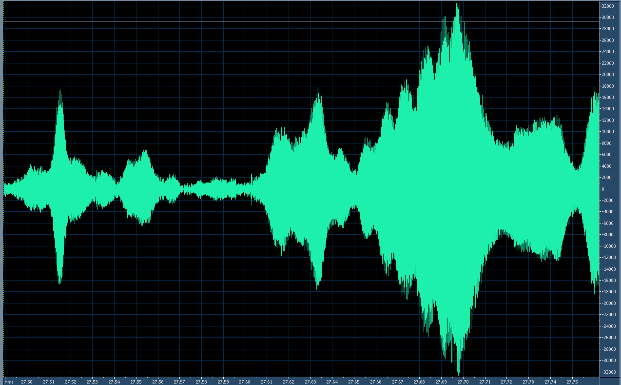
Figures 4 and 5, below, depict the rapid amplitude variations using a transmitted 4 kHz tone as an amplitude reference over a "Free Space Optical" path of approximately 15 miles (24km).  The horizontal axis is time and the vertical axis is linear amplitude.

Note the difference in horizontal time scales between the depictions, below:

Figure 4:
Scintillation of the laser-transmitted audio (4 kHz tone).
The time span of this particular graph is just over 250 milliseconds (1/4 second)
Click on the image for a larger version.

Figure 5:
Scintillation on the LED-transmitted audio (4 kHz tone).
In contrast to the image in Figure 4, the time span of this amplitude representation is nearly 10 times
greater - that is, approximately 2 seconds.  The rate and amplitude of the scintillation-caused
fading are dramatically reduced.
Click on the image for a larger version.

Laser scintillation:

As can be seen from Figure 4 there is significant scintillation that occurs at a very rapid rate.  The reference of this image is, like the others, based on a full-scale 16 bit sample.  Analysis of the original audio file reveals several things:

• While the "primary" period of scintillation is approximately 10 milliseconds (100Hz) but there is evidence that there are harmonics of this rate to at least 2.5 milliseconds (400 Hz) - but the limited temporal resolution of the test tone makes it difficult to resolve these faster rates.
• Other strong scintillatory periods evident in the audio sample occur at approximate subharmonics of the "primary" scintillatory rate, such as 75 and 150 milliseconds.
• The rate-of-change of amplitude during the scintillation is quite rapid:  Amplitude changes of over 30 dB (a factor of 1000) can occur in just 20 milliseconds.
• The overall depth of scintillation was noted to be over 40dB (a factor of 10000) with frequent excursions to this lower amplitude.  It was noted that this depth measurement was noise-limited owing to the finite signal-noise ratio of the received signal.

LED scintillation:

Figure 5 shows a typical example of scintillation from the LED using the same size emitter aperture as the laser.  Analysis of the original audio file shows several things:

• The 10 millisecond "primary" scintillatory period observed in the Laser signal is pretty much nonexistent while the 20 millisecond subharmonic is just noticeable.
  
• 150 and 300 millisecond periods seems to be dominant, with strong evidence of other periods in the 500 and 1000 millisecond range.
• The rate-of-change of amplitude is far slower:  Changes of more than 10 dB (a factor of 10) did not usually occur over a shorter period than about 60 milliseconds.
• The overall depth of scintillation was noted to be about 25 dB (a factor of about 300) peak, but was more typically in the 15-18dB (a factor of 32-63) area.

One of the more interesting results of this experiment was how minimally the severe amplitude distortion experienced with the laser actually degraded the overall intelligibility of human speech.  While the tones and brief music clips were clearly badly distorted, it could be argued that with the segment including speech, the degree of that distortion was not as apparent.  Clearly the voice content was being badly "chopped up" by the severe amplitude fluctuations, but with the redundant nature of speech and the fact that the drop-outs were quite brief in comparison to the duration of speech elements (sounds, syllables) it is quite reasonable to be able to expect the brain to fill in the gaps and make sense of it all.

A "Scintillation Compensator":

Despite the redundant nature of the speech maintaining reasonable intelligibility, it became quite "fatiguing" to listen to audio distorted in this manner so another device was wielded as part of an experiment:  The "Scintillation Compensator", the block diagram being depicted in Figure 6, below.

Figure 6:
Block diagram of the "Scintillation Compensator" system.
Click on the image for a larger version.

This system is essentially a "Keyed AGC" system using a low-level 4 kHz tone from the transmitter as an amplitude reference for a tracking gain cell at the receiver:  If the amplitude of the 4 kHz tone being received from the distant transmitter goes down, the gain of the audio in the receiver is increased by the same amount and vice-versa.  The effect of this device is quite dramatic as the clip in Figure 7, below, demonstrates:

Figure 7:

Audio clip with a"Before" and "After" demonstration

of the "Scintillation Compensator" 
Music:  "Children" by Robert Miles, used
in accordance with U.S. Fair Use laws.

One of the more striking differences is that in the "before" portion, the background hum from city lights remained constant while in the "after" portion it varied tremendously, more clearly demonstrating the degree of the amplitude variation being experienced.  What is also interesting is that the latter portion of the clip is much "easier" (e.g. less fatiguing) to listen to:  Even though syllables are lost in the noise, being obliterated by hum rather than silence in the first part of the above clip, the fact that there is something present during those brief interruptions, even though it is hum, seems to appease the brain slightly and maintain "auditory continuity".

It should be pointed out that the "Scintillation Compensator" cannot possibly recover the portions of the signals that are too weak (e.g. lost in the thermal noise and/or interference from urban lighting) but only that it maintains the recovered signal at a constant amplitude.  In the first portion of the clip in Figure 7 it was the desired signal level that changed while in the second portion it was the background noise that changed.  In other words, in both examples given in Figure 7, the instantaneous signal-to-noise ratio was the same in each case.

Practical uses for all of this stuff:

The most important point of this exercise was to demonstrate that a larger aperture reduces scintillation - although that point might be a bit obscured in the above discussion.  What was arguably more dramatic - and also important - was that the noncoherent light source seemed to be less susceptible to the vagaries of atmospheric disturbance.  This observation bears out similar testing done over the past several decades by many others, including Bell Labs and the works of Dr. Olga Korotkova.

For a brief bibliography and a more in-depth explanation of these effects visit the page "Modulated Light DX" - LINK - particularly the portion near the end of that page.

The reduction of scintillation has interesting implications when it comes to the ability to convey high-speed digital information across large distances using free-space optical means under typical atmospheric conditions.  Clearly, one of the more important requirements is that the signal level be maintained such that it is possible to recover information:  Too low a signal, it will literally be "lost in the noise" and be unrecoverable.

As the demonstrations above indicate, the "average" level may be adequate to maintain some degree of communications, but the rapid and brief decreases in absolute amplitude would punch "holes" in data being conveyed, regardless of the means of generating or detecting the light.  Combating this would imply the liberal use of techniques such as Forward Error Correction (FEC) and interleaving of data over time - not to mention some interactive means by which "fills" for the re-sending of missing data could be automatically requested.  The "'analog' analog" to these techniques is the aforementioned ability of the human brain to "fill in" and infer the missing bits of information.

While lasers are well-known to be "modulatable" at high rates, doing so for LEDs is a bit more problematic due to the much larger device (die) sizes and commensurate increase in device capacitance.  To rapidly modulate an LED at an ever-higher frequency would also imply an increase of "dV/dT" (e.g. rate of voltage change over time) which, given the capacitance of a particular device would also imply higher instantaneous currents within it, effectively reducing the average current that could be safely applied to it.  What this means is that it is likely that specialized configurations would required (e.g. drivers with fast rise-times at high current; structurally-small, high current/optical density LEDs etc.) to permit direct modulation of very high (10's of megabits) data rates.

Using the aforementioned techniques has rather limited utility when the free-space optical links extend out to many 10's of miles/kilometers owing largely to the vagaries of the atmosphere and the practical limits of optical flux with respect to "link margin" (e.g. the need to use safe and sane amounts of optical power to achieve adequate signal to recover information - particularly as the rate of transmission is increased) but it may be useful for experimentation.

Additional information on (more or less) related topics:

• Throwing One's Voice 95 miles on a lightbeam - link  - Details of experiments with high-power LEDs over a 95 mile (152km) optical path
• Voice on a Laser Beam - link - General information about using PWM techniques for Laser diode (and LED) modulation
• Gate Current in a JFET - link - The development of a highly-sensitive optical receiver that utilizes JFET gate current.
• The "Modulatedlight.org" web pages - link - This collection of web pages offers a large resource for many things related to free-space optical communications, including experiments, equipment and links to other related sites.
• For more information about the "Scintillation Compensator" and the "Audible S-Meter" used to set up the optical links, look at the page "An Audio Interface Device for Speech Bandwidth Optical Communications" - link

[End]

This page stolen from "ka7oei.blogspot.com".

Gate current in a JFET: The development of a very sensitive, speech-frequency optical receiver.

Back in 2007-2008 I was working on equipment for "new" ham band - for me at least - the one that is now labeled as "...above 275 GHz" in the FCC rules.  As you might expect the most accessible portion of this infinity of electromagnetic spectrum is that containing visible light, and that is where I was directing my interest.

At this time "high power" LEDs were starting to appear on the market at reasonable prices, and by "high power" I mean LEDs that were capable of dissipating up to 5 watts, each.  What this meant was that from a single emitting die of rather small dimensions one could pump into it enough current and, with the good efficiency of the device, obtain a quantity of light that was suitable for long-distance optical communications.

To be sure, I was building on the fine pioneering work of others, including that of two Australians, Dr. Mike Groth (VK7MJ) and Chris Long (now VK3AML) who had determined that it was the noncoherent light produced by LEDs that offered the greatest probability of practical, very long-distance atmospheric optical communications.  (As a primer as to why this is the case, read the article Optical Communications Using Coherent and Noncoherent Light - link).

Optical receiver needed:

In the midst of producing the various pieces of equipment required for experiments in optical communications (e.g. optical transmitters, modulators, receivers, support equipment, etc.)  I was investigating the different circuit topologies of practical optical detectors.  My goal was not to achieve extremely high data speeds, but rather to use audio-frequency signalling (speech, tones) to start with and, perhaps, work up from there.

One of most common such detectors is the phototransistor - but I quickly dismissed that owing to its very small photoactive area and the fact that the various pieces of literature relating to weak-signal optical detection noted that they are inferior in comparison to practically any other device owing to their intrinsic noise level.  (CdS cells - article here -  were not seriously considered because they are too slow to respond - even for audio frequencies.)

One option was the venerable Photomultiplier Tube (article here) and while this was technically possible and, in theory, the best choice, it was ruled out because of its fragility (electrically and mechanically), its large size, the limited response at the wavelengths of interest (more below on that) and the need for a high voltage supply (around 1000 volts).

While these technical difficulties are surmountable I could not overlook the fact that available literature on these devices - and advice from the Australians, who'd actually used them - pointed out that there were but a few photomultipier tube types that have good sensitivity in the "red" end of the optical spectrum where there is also good atmospheric transparency - and even fewer of these rare types, in known-usable condition, available for a reasonable price on the surplus market!

Figure 1: 
The transimpedance amplifier in its simplest form. 
This circuit converts the photodiode currents
into a proportional output voltage.

The Transimpedance Amplifier:

This left me with the photodiode (article here) and the most commonly-seen circuit using this device is the "TIA" - TransImpedance Amplifier (article here).  As can be seen from Figure 1 this is very simple, consisting of just an operational amplifier with a feedback loop with the photodiode connected directly to the noninverting input.  In this circuit the photodiode currents are converted directly to voltage (hence the name) with the gain set by the feedback resistor with the added capacitor being used to assure stability, compensating for photodiode and op-amp capacitance.

This particular circuit has the advantage that it is very predictable and the frequency response can be determined by the combination of the bandwidth of the op amp and the intrinsic capacitance of the phototransistor.  To a degree, one can even increase the frequency response for a given set of devices by reducing the feedback, but this comes at the expense of gain and ultimate sensitivity.

In other words:  With photodiodes you can have high sensitivity, or you can have wide bandwidth - but not both!

Figure 2:
 A practical, daylight-tolerant TIA optical receiver circuit.  This has good sensitivity in both darkness and light and does not suffer from "saturation" in high ambient light conditions because of a built-in "servo" that self-adjusts the phototiode's virtual ground to offset photon-induced bias currents.  Because of this "servo" action this receiver does not have DC response like the circuit of Figure 1 with the low-end frequency being limited by the values of R104 and C106.
While the LM833 is a reasonable performer, there are other (more expensive!) op amps that have lower noise.
Click on the image for a larger version.

While very simple (there are even single-chip solutions such as the "OPT101" that include the photodiode, amplifier, and even feedback resistor in a clear package) there are some very definite, practical limitations to the ultimate sensitivity of this sort of circuit if the goal is to detect extremely weak, low-frequency currents.  When you get to very low frequencies, "1/f" noise (a.k.a. "flicker noise") becomes dominant from a number of sources and there are various other types of noise sources (thermal, shot, etc.) that can be produced by the various components.

As it turns out, this circuit - with practical op amps - has very definite limitations when it comes to trying to divine the weakest signals at low-ish frequencies (audio, sub-audio):  For an article on why this is so - and some of the means of mitigation - see the January, 2001 Electronic Design article, "What's All This Transimpedance Amplifier Stuff, Anyway?" - link by Robert Pease.

Figure 3: 
The VK7MJ optical receiver using TIA and cascode techniques - used as the "reference" optical detector.
The optional "daylight" circuit provides AC coupling to prevent saturation of the circuit under high ambient
light conditions at the expense of low-light performance.
Click on the image for a larger version.

One can build transimpedance amplifiers using discrete components that outperform most of the integrated-circuit based designs and for a reference circuit I constructed and used one devised by Dr. Groth, VK7MJ and depicted in Figure 3.  In this circuit one may see the feedback path via R3/R4 with compensating capacitor Cf.  In this particular circuit Q1, the input FET, is rather heavily biased to increase its "bulk current" (a term used in the referenced Robert Pease article) with Q2 acting as a cascode circuit - link (e.g. current-based) amplifier with subsequent follower stages.  Additionally, the photodiode itself (D1) is reverse-biased, reducing its capacitance significantly and thereby improving high frequency response.  By hand-selecting the quietest JFETs one can obtain excellent performance with this circuit and since it is discrete, there is room for adjusting values as necessary to accommodate component variations and for experimentation.

This particular circuit is quite good across the audio range from a few 10's of Hz to several kHz, but above this range it is largely the capacitance of the photodiode (at least for devices that have square millimeter-range surfaces areas) that quashes the high frequency response.  Even though the photodiode's capacitance - and that of stray wiring and the JFET itself - may be only in the 10's of picofarads, at hundreds of k-ohms (or megohms) even small amounts of capacitance quickly become dominant - another good reason to implement the aforementioned cascode circuit and its tendency to minimize the "Miller Effect" - link to help optimize frequency response.

The K3PGP circuit and variations:

Figure 4: 
The K3PGP Optical receiver.
Click on the image for a larger version.

Building the above circuit as a "reference" I began testing on a "Photon Range" - a darkened room in my basement with a red LED affixed to the ceiling - where I characterized the various receiver topologies.  In this environment a small and adjustable amount of current (10's of microamps, typically) would be fed to the LED, modulated at an audio frequency, and the receiver under test would be placed on the floor below with its output connected to a computer in an adjacent room running an audio analysis program such as "Spectran" or "Spectrum Lab" to measure the signal-noise ratio at different frequencies.  Before and after each session I would measure the performance of my "standard" optical receiver - the VK7MJ circuit - and use it as a basis of comparison.

The receiver named after K3PGP (see his web site - link) was the next receiver to be tested.  This receiver is much more sensitive than the VK7MJ receiver - at least at very low audio frequencies (<200 Hz) and as may be seen in Figure 4 it is devoid of a feedback mechanism and the connection between the photodiode and JFET is made directly, with no external biasing components of any kind.

While a seemingly simple circuit, there is more going on here than one might first realize:  Without any feedback or any other components between the FET and photodiode the opportunity to introduce noise from such components or reduce the signal from the photodiode in any way is minimized.  In fact, when constructing this circuit there is the strong admonition that the photodiode-gate connection to the JFET be done in mid-air (and that one clean both components with alcohol to remove residue!) as leakage paths on circuit board material can cause significant signal degradation!

Effectively, the K3PGP circuit acts as a charge integrator with the energy slowly (in relative terms) bleeding off due to the leakage of the photodiode, its photoconductivity, and the gate-source leakage currents of the FET itself.  While extremely sensitive at low frequencies - specifically those below 200 Hz - above this, the sensitivity and output suffers due to the rather long R/C constant associated with the high gate-photodiode leakage resistance and capacitance and, to a lesser degree, the Miller effect.  This circuit also functions only in total and near-total darkness conditions:  More light than that, the voltage across the photodiode reaches equalibrium while turning the FET "on", effectively quashing the signal.

Inspired by the above circuit I made the modification indirectly depicted in Figure 5, below:

Figure 5:
 The version "2.02" optical receiver, used as a test bed for various circuit configurations - see text.
For the "K3PGP" configuration the photodiode would be reversed from what is shown
in the drawing above and the anode grounded with nothing else connected at point "C".
Click on the image for a larger version.

This circuit was devised as a "test bed" and although not shown in the diagram, it was configured by connecting the cathode of the photodiode to the gate and grounding the anode and having no other photodiode-gate connections present - just as in the K3PGP receiver.

In this circuit one has a FET input and a cascode circuit - just like that of the VK7MJ circuit - to reduce the Miller effect, but this particular cascode circuit has a modification:  Q3 forms a current source, in parallel with the cascode, that supplies the bulk of the drain current for the JFET - several milliamps.  Because the amount of current provided by the current source - which has a high operating impedance and is largely "invisible" - is fixed (but adjustable by varying R4 to suit specific characteristics of Q1) and it is left up to the cascode to supply the remaining drain current - which varies depending on the gate voltage.  In this particular circuit, due to the "cascode action" the voltage at the drain of Q1 and emitter of Q2 varies very little while the cascode - which is allowed to bias itself at DC, but is bypassed at AC with C3 - produces the recovered modulation at the collector of Q2, greatly amplified.  From the collector of Q2, noninverting amplifier U1a amplifies the signal further and presents a low-impedance output.

In other words, it is mostly the K3PGP circuit, but with a cascode amplifier and higher FET drain current:  By reducing Miller capacitance with the cascode the frequency response was to be improved somewhat and by increasing the drain current the noise contribution of the FET itself should be reduced as noted in the Pease article mentioned above.

In testing it was observed that this particular circuit was, in fact, several dB more sensitive than the original K3PGP circuit and also that the frequency response was slightly better - but not as much as one might first think, mostly owing to the fact that it is mostly the photodiode capacitance that is limiting the response rather than the Miller effect - but every little bit helps!

I then rewired the circuit using the "Standard Config" noted in Figure 5 which, if you draw in the lines, converts it into a TIA circuit like that of the VK7MJ design with both adjustable reverse bias of the photodiode and adjustable feedback.  In this configuration the performance at very low frequencies was reduced, likely due to the noise contribution of the feedback resistor, increased leakage currents from the photodiode at reverse bias and also signal attenuation caused by the feedback submerging the lowest-level, low-frequency signals into the noise.  At "speech" frequencies it was slightly better than that of the VK7MJ receiver - probably due to the higher JFET current or, perhaps, random component variances - and the frequency response was also comparable to that of the VK7MJ circuit, the parameters varying according to the amount of applied feedback and compensation.

Improving the receiver:

My goal was a circuit that offered the sensitivity of the K3PGP circuit, but usable speech response - the latter not being available from the K3PGP circuit due to the R/C rolloff.  A quick check revealed that this was the typical 6dB/octave rolloff so I reconfigured the circuit, again, as a K3PGP-like circuit and followed it with an op-amp differentiator circuit with a breakpoint calculated to compensate for the measured "knee" frequency (e.g. that at which the 6dB/octave rolloff of the K3PGP circuit) began - the result being that I now had a fairly flat frequency response.  Not unexpectedly, while the signal-noise ratio was quite good at the very low frequencies, it decreased fairly quickly as it went up as that energy was simply submerged in the circuit noise.

In staring at the circuit, with the grounded anode of the photodiode, I wondered about reverse-biasing the photodiode to reduce the capacitance - but if I did this, how would I keep the voltage at the gate from rising without needing to add another (noise generating, signal-robbing) component to clamp it to ground?  Knowing that the gate-source junction of a JFET was much like that of a bipolar transistor in that there would be an intrinsic diode present, I knew also that the gate-source voltage would limit itself to 0.4-0.6 volts, but how would the FET behave?

Using JFET Gate current for "good":

In doing a bit of research on the GoogleWeb when I derived this circuit I could not come up with any sort of useful answer to the "gate current" question, so I simply did it, constructing a "gate current amplifier":  The photodiode was reverse-biased with the minute leakage, dramatically reducing its capacitance, and photoconducting currents being sinked by the gate-source junction.  As expected, the drain current increased noticeably, but the circuit worked extremely well, with both frequency response and apparent gain increasing dramatically!

Putting this "new" circuit back on the photon range I observed that although its low frequency (<200 Hz) sensitivity was slightly worse than that of the K3PGP circuit (see comment below), the higher speech-range frequencies (300-2500 Hz) were, on average, 10-12dB better than the VK7MJ circuit and approximately 20 dB better than the best, low-noise op-amp based TIA circuit that I'd built to date!

In analyzing the circuit, there are several things happening:

• Reverse bias of the photodiode:  This reduces the capacitance - typically by a factor of 3-6, depending on the specific device and voltage applied.
• The photodiode will produce current in the presence of light.
• Being reverse-biased, the photodiode will also operate in a photo-conductive mode, passing current from the bias supply in response to light.
• With the gate-source junction conducting, the reverse bias across the photodiode is maintained since the gate-source voltage will never exceed 0.4-0.6 volts.
• As described above, the amplifier is connected in "cascode" configuration to minimize Miller effects.
• There are NO other components or signal paths connected to the photodiode-gate junction that can contribute noise or attenuate the signals.
• In parallel with the cascode circuit is a current source which provides a high-impedance current source to increase the JFET's bulk currents, further reducing its noise.

 About the gate-source conductivity of the JFET, two things surprised me:

• The "diode action" of the gate-source clamping seems not to be a significant contributor of noise - at least at "dark" currents of the photodiode.
• There is little or no documentation about using a JFET this way, anywhere else!

It is likely that the main reason that this doesn't perform quite as well at the K3PGP circuit at low (<200 Hz) frequencies is because of the intrinsic leakage current noise endemic to the reverse biasing of the photodiode, particularly in a "1/F" manner:  At higher frequencies where this sort of noise falls away it performed far better. 

Note:

In "photon range" testing it was difficult to tell at which frequencies the K3PGP receiver performed better.  My K3PGP exemplar receiver was certainly better at, say, 20 Hz, but even at 100 Hz or 60 Hz it was a difficult call to make.  At such frequencies and under such conditions careful selection of the "quietest" photodiode and FET can make a significant difference and with most of these circuits, reducing their temperature - while somehow managing to avoid condensation - can help even more!

Plotting Gate current versus Drain and Gate voltages:

Later, I constructed a test fixture to analyze the gate-source voltage and gate-source current response of a 2N5457 JFET and plot this against the drain current - see Figure 6 below.

Figure 6:
 Gate-source voltage and Gate current plotted against drain current for a typical, real-life JFET - not a simulation!  Note the logarithmic scale of the gate current and also that the drain current continues to increase linearly with gate-source voltage, even after the gate-source junction is conducting.
Click on the image for a larger version.

As can be seen, as the gate-source voltage increases, the drain increases linearly - even after the gate-source diode junction starts to conduct:  In fact, there does not appear to be inflection of the drain current curve when this happens!  Following the other line representing gate current we can see that once our gate-source "diode" starts to conduct, the gate current follows the classic logarithmic curve that one associates with diodes - which should not come as a surprise.

Equation 1:
The relationship between drain current and
gate-source voltage.
Vgs= Gate-source voltage
Vp=FET Pinch-off voltage
Idss=Zero gate voltage drain current

According to typical JFET models, in the saturation region the FET operates such that the drain current is generally independent of the drain voltage as can be seen in Equation 1 and the graphs in Figure 6 indicate that this seems to be true even when the gate-source junction is conducting.

So, now we know what is happening.  At first glance, one might presume that with this diode in conduction that the logarithmic response would make the circuit unsuitable for general audio recovery - but this is not so:  At very low light levels the detector has lower than 1% harmonic distortion.

Figure 7:
Test circuit used to derive the curves in Figure 6.
For measuring the voltage at "Vgate Monitor" it will be
required that the negative lead of the voltmeter be referenced
to a regulated, negative (with respect to ground)
voltage source.  Q1 is the device being tested and
Q2 is just another JFET which need not be the
same type as J1.

In case you are interested, Figure 7 shows the circuit that was used to derive the curves in Figure 6, above.  10.0 volts was used for V+ and the drop across source-follower Q2 was easily characterized so that the drop across R1 - and thus the gate current in Q1 - could be determined.  The drain current was determined by measuring the voltage across R2.  Different values of R1 were used to achieve the measurement range depicted in Figure 6 which accounts for the very slight bend in the "Gate Current" curve.

Putting this into practice:

The circuit depicted in Figure 8 was developed for speech-bandwidth optical communications use.

As can be seen, this looks very similar to the circuit of Figure 4 with the exception that the reverse-biased photodiode is connected to the JFET and that there is the added circuit, U1b, that forms a bandwidth-limited differentiator - the component values chosen to approximately correlate with the low-frequency "knee" of the BPW34 photodiode and also to cease its frequency boost above 5-8 kHz.  (The "Flat" audio output, uncompensated by the differentiator for the 6dB/octave rolloff, is provided for both very low frequency - below 200 Hz - and high frequency - above 5 kHz - signals to be applied to a computer for analysis.)

The circuit in Figure 8 - and minor variations of it - have been replicated many times over the years using different components.  The important considerations are that both Q2 and Q3 be low-noise, high-beta transistors such as the MPSA18 (or 2N5089) and that the JFET used for Q1 be capable of rather high drain current.  In the original design, the 2N5457 was specified as this device is better-characterized that many other, similar FETs and is capable of quite low-noise operation:  The more common MPF102, with its extremely wide variation of parameters, might be suitable if an appropriate device is "cherry picked" from amongst several based both on high zero gate-source voltage drain current and tested "noisiness".  A more modern JFET is the BF862 - available in surface-mount only (as are most JFETs these days!) - that is even better for this application than the 2N5457 and capable of much higher drain ("bulk") current to the point where utilizing its full potential might compromise 9-volt battery life!

Figure 8:  
Version "3" of the optical receiver.  This receiver must always be operated on its own, completely isolated power supply to avoid feedback.  V+ is 8-15 volts and is typically a 9-volt battery.  D4 and TH1 prevent damage should the applied polarity of the power source be accidentally reversed.  After Q1's drain current has been measured and adjusted, jumper "J1" is closed.
A version of this circuit by the author of this page also appeared in an article published in the SPIE proceedings (#6878) which was presented at the 2008 "Photonics West" conference by another one of the paper's co-authors, Chris Long.
Click on the image for a larger version.

In a circuit such as Figure 8, above, the drain-source voltage will be much lower than one might initially expect - on the order of 0.2-1.0 volts for a JFET such as a 2N5457 and between 0.1 and 0.5 volts for the BF862 - but this is normal operation.  While the setting for Q3 current, adjusted via R5, (in Figure 8) at 120 ohms is suitable for most 2N5457 devices, the current may need to be reduced (e.g. R5 increased in value to 180 or 220 ohms) for some "lower 0 Vgs" current devices such as the MPF102.  In general, the higher the drain current, the lower noise contribution from the FET - but if you exceed the "magic" value and attempt to force too much current, the circuit will suddenly stop working:  Overall it is better to have a bit lower drain current than optimal and have a little bit more noise than to have too much drain current!  (Don't forget that the properties of the current source and the JFET itself will also change with temperature - but they generally seem to track.)

Interestingly, the circuit depicted in Figure 8 also works in daylight, albeit with some caveats.

When very high levels of light are present, the photoconductivity will shunt the reverse bias to the gate-source junction, and the frequency rolloff "knee" associated with the photodiode capacitance will shift upwards due to photoconductive shunting causing the audio to become "tinny".  The audio will also become somewhat distorted owing to the different light-to-audio transfer curve that occurs under such conditions, in which case the frequency response of the audio on the "flat" output is more suitable than otherwise.  In such situations one does not really need the high sensitivity of this type of receiver, anyway, and a typical TIA circuit with AC coupling such as that depicted in Figure 2 or Figure 3 could be used or one could apply optical attenuation in front of the detector to reduce the light level.

Practical use:

Figure 8:
An as-built "Version 3" optical receiver, constructing using
prototyping techniques and enclosed in a shielded, light-tight
enclosure using pieces of printed circuit board material.  For this
unit "feedthrough" capacitors are used for power and audio
connections to prevent the incursion of RF energy on
the connecting leads.
Click on the image for a larger version.

Entire web pages could be written (and have been - see the Modulated Light web site - link) about through-the-air, free-space optical communications over long distances (well over 100 miles, 160km) using both LEDs and low-power lasers, but even the most sensitive receiver - no matter the underlying technology - requires supporting optics (lenses!) in order to function properly:  It is through such lenses that 10's of dB of noiseless signal gain may be achieved, not to mention directionality and the implied rejection of off-axis light sources.

The circuits described on this page are likely to be suitable only for speech frequencies and low-rate data but this is, in part, due to the medium involved (the atmosphere) and method of transmission.  At the extreme distances that have been achieved with the above equipment (>173 miles, 278km) the signals are weak enough that only low-rate signalling techniques would likely be feasible under typical conditions at safe, practical optical power levels.

Additional web pages on related topics:

• Modulatedlight.org - This web site has a wide variety of information related to amateur, free-space optical, through-the-air communications.
• Optical Receivers for Low-Bandwidth, Through-the-Air Communications - This is a reference article that gives additional detail about the design of the circuits discussed in this article.
• Using Laser Pointers for Free-Space Optical Communications - This describes how one might use low-power laser pointers for low-rate optical communications, the practicalities of various circuits, the methods and the realities.
• The Modulated Light DX page - This page has several articles describing the practical aspects of free-space, through-the-air optical communications including various atmospheric effects.
• A description of this circuit appeared in the SPIE Conference Proceedings, Volume 6878, “Atmospheric Propagation of Electromagnetic Waves II” in the article "Dollars versus Decibels:  Long-Range atmospheric optical communications on a tight budget".  This article was presented at the January, 2008 Photonics West conference and a copy of this article may be read here.

The above web pages also contain links to other, related pages on similar subjects.


[End]

This page stolen from "ka7oei.blogspot.com".

Updated version of the "Simple" PWM LED/Laser modulator

A few years ago, for our friends in the Tucson area, I threw together a "simple" PWM circuit for audio modulation of high power LEDs (but it works just as well for laser pointers) for an optical transmitter - you can read about that here:

A "Simpler" Pulse-Width Modulator for LEDs, Lasers and whatnot and a simpler foam-core enclosure - link

Figure 1:
As-built prototype of the updated PWM transmitter designed to test both
 the AGC and manual gain/tone configurations.
There is currently no circuit board pattern:  If you design one,
please let me know!
Click on the image for a larger version.

As the page describes, this was intended to be comparatively simple and flexible in its operation, providing both modulation of both audio and test tones.  While it worked just fine, it did bother me a bit that it did not have a "manual" gain mode - that is, one could not simply override the audio AGC - which does work quite well - and "ride" the audio level manually, instead.

That was 2009 - so flash forward to 2014 when, at the request of some fellow amateurs in Australia, I finally got the impetus to update the firmware to add the means of selecting a completely manual gain control to the PWM circuit, of so-desired, in addition to various tone modes, all by setting pins on the PIC processor to the appropriate logic levels.  Of course, the original AGC audio mode is still present and may be used exactly as before, if one wishes, and one could even construct the circuit so that it could be switched between manual and AGC mode.

What it's for:

If you have ever been to the Modulatedlight.org web site link  (which I'll admit to having quite a lot to do with...) you will know that it has a lot to do with optical communications - mostly using high-power LEDs, but it also touches a bit on using low-power laser modules as well.

For modulating audio onto LEDs, onto LEDs, one of the easiest ways to do this is via linear current modulation, a process that is explained on the web page Linear Modulator for high-power LEDs - link.

Figure 2:
Examples of waveforms used to generate PWM signals,
from the web page "The Luxeon:  
New Light of Hope for Optical Communications"
by Chris Long

Another way that LEDs may be modulated is by turning them on and off in a manner that simulates linear modulation using a method called PWM, or Pulse Width Modulation - a system that is very easy to do using digital hardware such as counters and is often found in microcontrollers.

For laser diodes such as those found in laser pointers, current modulation is NOT very good for a number of reasons, including the fact that the brightness-current curves of laser diodes isn't particularly linear over a wide range, nor is it predictable at which current a diode will start to laser under a given set of conditions (e.g. temperature, age) or up to what current a specific diode can be safely operated!

For amplitude modulation, it is always preferable that one modulates as deeply as possible to achieve the best-possible signal-noise ratio and if one is trying to current-modulate a laser diode, this becomes problematic as the bounds of safe and reliable operation are difficult to know!  It is more convenient, then, to simply turn it on and off, operating it at a known, safe current when it is on and varying the duty cycle using PWM.

If the switching frequency of the PWM is sufficiently high it will be compatible with a "conventional" analog optical receiver that was intended for amplitude-modulated light sources as the PWM waveform will be integrated by the low-pass response of the receiver's front end.  At the very least, the PWM frequency must be at least twice that of the highest modulating frequency of the audio to be carried  and if necessary, a simple low-pass filter could be added to an existing receiver to remove any residual switching components - see Figure 2 for a pictorial of how a "slow", low-pass response can smooth out the PWM frequency components.

How it works:

Figure 3:
Diagram of the version with audio AGC.
Click on the diagram for a larger version.

This circuit uses a PIC12F683, an 8 pin microcontroller internally clocked at 8 MHz.  Using its PWM hardware, it generates a waveform with a clock rate of 31.25 kHz that is pulse-width modulated at a resolution of 8 bits - suitable for voice.

Audio can come from one of two places:  A built-in tone generator, or an external microphone/line-in audio source.

Using DDS techniques, audio sine waves can be generated at frequencies from a few 10's of Hz to several kHz and these are applied to the PWM generator, producing tones with 100% modulation depth.

Audio from the microphone or line input is first amplified and then low-pass filtered to remove high-frequency content and applied to the 10 bit A/D input of processor where it is digitized at a rate of 31.25 kHz and also passed to the PWM output.

"AGC" mode:

In diagram depicted in Figure 3, the circuit is configured to use an audio AGC to assure that the modulation is kept at a consistently-high level.  The audio level is monitored continuously to determine if its level is within 6 dB of clipping.  If it exceeds that level, a counter is incremented, but if it does not, a counter is allowed to self-decrement.  If the counter exceeds a pre-set value indicating that the audio level has been high recently, the processor pins that control the gain on the amplifier stage are adjusted to reduce the gain to the next, lower step.  If the counter self-decrements below a pre-set value indicating that the audio level has been consistently low, the gain is adjusted to increment.

There is also a built-in 12 dB gain adjustment in software:  If the audio has been low and the audio gain is near maximum, a 12 dB gain step can be switched in which is done by first limiting the A/D values in software to ostensible 8 bit values and then shifting the A/D data to the left by two bits and offsetting.

When switched to the "tone" mode, instead of audio being applied to the A/D input, the voltage from potentiometer R220 is applied instead allowing a variable voltage to be used to set the tone mode:

• <=0.5 volts:  1 kHz tone
• >0.5 to < 4.5 volts:  Variable frequency audio tone
• >= 4.5 volts:  Tone sequence

Having a fixed 1 kHz tone is useful if using a computer or other device when setting up end-to-end alignment of an optical path as narrow detection bandwidths may be employed to maximize the overall sensitivity of the detection scheme.  Because this PIC's oscillator is not crystal-based, the actual frequency can vary by several percent, but it should be easily spotted with spectral analysis programs such as "Spectrum Lab" by DL4YHF, Spectran or Argo (to name but a few).

In the variable tone mode the frequency may be set from a few 10's of Hz (below mains frequency) to a bit over 2 kHz as desired.  Finally, the "tone sequence" mode is designed to emit a musically-dissonant series of notes (C4, E5#, F4#, E6) that really stick out of the noise:  By being dissonant, spanning over an octave and non-continuous they avoid "ear fatigue" and are more likely to be heard amongst other sounds that may be being heard from power mains and electric signage that might be intercepted.

Manual gain mode:

Figure 4:
The version with manual gain control
Click on the image for a larger version.

While the audio AGC works quite well to assure that ones voice fully modulates the LED to maximize "talk power" and signal-to-noise ratio, one may prefer to have a manual gain control instead and manipulation of several of the pins on the processor allows the selection of that mode as depicted in Figure 4.

In this version the audio gain is set with R309, but one can effect a "software" gain setting two switch in an extra 12 dB of gain via appropriate strapping of pin GP4.  As with the "AGC" version, there a variable "tone" mode is available but there are also some "fixed" tone modes that may be selected via appropriate strapping of pins GP3, GP4 and GP5 if you don't wish to use a potentiometer.

Minimalist version:
 

Figure 5:
Minimalist version.
Click on the image for a larger version.

Finally, Figure 5 depicts a somewhat minimal approach to the circuit, using only a single op-amp section with no active low-pass filter, manual gain control and the optional selection of a tone mode if you choose to implement switch SW301.

At its very simplest, one would connect GP3 (pin 4) to the +5 volt line to put the PIC into audio mode all of the time, but the triviality of adding just one SPST switch and a resistor would provide the facility of a tone generator, doing so would be hard to resist!

Getting the code:

If you are interested in building a modulator for an LED or laser using this device and are interested in the .HEX file for programming the PIC yourself, please let me know.  If you don't have a way to program the PIC and want a pre-programmed device, I can arrange that, too.


More information:

For more information about Free Space Optical Communications for the amateur, be sure to visit the Modulated Light page - http://www.modulatedlight.org



[End]

This page stolen from "ka7oei.blogspot.com".

50 years since operation "Red Line"

It's hard to believe - especially, I am sure, for those who were involved - that it's been over 50 years since Operation Red Line.

For more details visit the Operation Red Line web site:  
 
http://www.modulatedlight.com/eos/Operation_Red_Line.html


What was Operation Red Line?

Back in early 1963 - just a few months after the invention of the visible Helium-Neon Gas Laser - a group of (mostly) amateur (ham) radio operators that happened to work at EOS (Electro-Optical Systems, later affiliated with Xerox/Parc) in Pasadena, California took on the challenge of doing something that would be both fun and challenging:  Go for the distance record for laser-beam communications.

A 1963 Laser

Figure 1:
On the workbench, the EOS Helium-Neon laser tube.  The Viking II
transmitter - the source of the RF excitation and modulation - may
be seen to the right of the laser.
Click on the image for a larger version.

At this time you couldn't just go out and buy a Helium-Neon laser tube, so they managed to cobble it and the optics together with the blessings of the senior management and a bit of help from their own well-equipped glassblowing and optics shops.

One of the vexing problems with early gas lasers - or practically any gas-discharge tube - was that of contamination/wear of the electrodes used to excite the gas mixture within the laser tube, so rather than mess with trying to engineer a solution to yet another problem, they chose electrode-less RF excitation.

But first, they had to get it to work!

The RF source itself was pretty easy:  Being ham operators, they already had access to a 100-watt class AM transmitters so Bob Legg, W6QYY, offered the use of his Johnson Viking II transmitter.  They chose a 10 meter frequency of 28.620 MHz, because it was a rather high frequency and would make the matching a bit easier, but it would also be more likely to couple into the tube and properly excite the gas - plus there was less chance that the 10 meter band would be open and the unintentional RF radiating from the coupling system would be heard halfway across the world!

In this case the idea was easy, but the implementation was more difficult:  How does one properly excite the gas inside the tube so that it lases?  Electrodes on the glass in the form of self-adhesive copper tape were an obvious choice, but it turned out to be a bit of a challenge to achieve uniform excitation until someone struck on the idea of interleaving elements, with every other element connected together, fed 180 degrees out of phase with the other set via a balanced-wire output from the transmitter coupling.

Finally, lasing!

Figure 2:
The "business" end of the laser, in the lab.  A pair of semi-silvered,
confocal mirrors were used to allow the laser to work.  The laser
assembly was put into a large piece of metal channel so that it
could be transported and maintain a degree of mechanical/optical
alignment.  A "10 power" telescope was used to collimate the
beam to approximately 2 inches (5 cm) diameter to minimize
atmospheric scintillation.
Click on the image for a larger version.

Even though around 100 watts of RF was being input to the matching network, the EOS folks were able to measure only about 125 microwatts of light emerging from the laser itself.  In speaking with those that were there at the time, they believed that with additional work they could have gotten more power out of the laser, but they felt compelled to get it out of the lab as soon as possible since crunching the numbers indicated that 0.125 milliwatts should be more than enough power to cover any distance for which they were likely to find a line-of-sight path!

The RF alone wasn't usually enough to "strike" the tube and cause the gasses within to ionize, but they had on hand a device that they referred to as a "zapper".  About the size of a high-power soldering iron, this gadget was used in the neon light and vacuum tube industry to test for gas within the device being tested by outputting a very high voltage, low-current arc that can ionize the gas within, through the glass via capacitance -  much like the trigger electrode of a xenon strobe tube:  This device is actually visible in Figure 1, sitting on the upper shelf on the far right, to the left of what looks like a water glass.

The mechanical adjustments for the laser were also very finicky.  At each end was a partially-silvered confocal mirror on a micrometer mount and it was very easy for slight temperature variations and flexure of the laser assembly to knock these out of alignment and prevent lasing.  As it turned out, both mirrors were identical so laser light was actually emitted from both the "front" and "back" of the laser, but this "wasted" laser energy from the back was useful in tweaking the laser while it was in operation since this could be done without blocking the light going to the distant end.

Finding a long, line-of-sight path:

Meanwhile, other members of the group were busy poring over maps to find two locations that were line-of-sight with each other and offered some hope of being accessible by vehicles that would be available for use and eventually, a pair of sites emerged as candidates worth checking out on the ground.  The west-ish end of the path, near the Grassy Hollow campground in the San Gabriel mountains and another site in the Panamint range, next to Death Valley and east-ish of the (almost) ghost town of Ballarat.

Getting to the Grassy Hollow site didn't appear to be too much of a problem:  Easy access from good roads near an established campground.  The Panamint site was more of a challenge, but making contact with the sole inhabitant of Ballarat - an old miner who called himself "Seldom Seen Slim" - and a few others that had mining claims in the area - proved fruitful and they were able to get permission to travel across these claims as well as get directions to some of the higher-elevation roads.  After a bit more scouting about they found a location along a road at which there was enough flat-ish area for both vehicles and setting up the gear and it offered a good view back toward Grassy Hollow.

The calculated distance?  A bit over 118 miles according to the maps.

Detecting a distant laser:

Figure 3:
In the lab, detecting the purposely-attenuated laser light using a 12.5-inch
reflector telescope.  This was one of many tests "in the lab" before the
gear was taken into the field.
Click on the image for a larger version.

At this point, one may start to wonder about the "other" end of the laser path.

It wouldn't do just to shine a laser from point "A" to point "B", but it was necessary to be able to communicate - if only one way - over the beam electronically, preferably via voice.  To do this, a means of detection of the (likely) weak beam was required.

Fortunately, one of their number, Parks Squyres, owned a large reflector telescope, a Herring-Cave 12.5 inch (approx. 32 cm) Newtonian.  To it they fitted an external box containing a movable front-surface mirror to direct the gathered light either to an eyepiece or an electronic light detector known as an S-20 "Photomultiplier" tube.  This type of tube, invented in the 1930's, is used today as it is still unsurpassed in its sensitivity to light and it was the natural choice at the time since there were no other types of electronic light detectors that came anywhere close to being sensitive enough for this task!

For testing they took advantage of the fact that the EOS building was laid out such that, using mirrors, they were able to send laser light - severely attenuated to attempt the simulation of atmospheric effects - up one hall and down the other, a distance spanning well over 100 feet.  After a bit of tweaking they were able to get good results transmitting voice from end-to-end of this simulated path, giving them confidence that the entire system would have a reasonable chance of working!

Modulating the laser was actually the "easy" part.  Originally, they had intended to take advantage of the polarized light of the laser itself (its design included a pair of "Brewster's Windows") and use a "Kerr Cell" - a device that can be used to electronically rotate the polarization at extremely high speeds - and using the two together it would theoretically be possible to convey many channels of voice.  In the interest of time and simplicity, however, they used the same Viking II transmitter that was providing the RF excitation to amplitude-modulate the light since it was, after all, an AM transmitter!    Because amplitude modulation (AM) RF was used for modulating the laser, some care had to be taken to avoid excessive excursions to "0%" modulation or else the laser would "go out" and require re-striking with the "zapper"!

Figure 4:
The laser at Grassy Hollow, set up in a tent.  Communications between this, the transmit site and the receive site
about 119 miles away was maintained using the 2 and 6 meter amateur bands.
Click on the image for a larger version.

Time was of the essence:

The EOS folks were on a bit of a "fast track" with this project because they got wind of at least two other groups making preparation to span a fairly long distance.  One of these was associated with Ryan Aircraft and other with the U.S. Military, both of whom were making rather elaborate preparations.  Since this was a purely volunteer effort using donated time, equipment and funds, there was the double pressure of making it work quickly and cheaply!

Soon after getting both the laser and receiver working they scheduled a weekend during which they would go out into the field and make a first attempt:  Friday, May 3, 1963.

Getting to the Grassy Hollow campground was fairly easy:  They just drove their cars and station wagons to the site, set up tents and then fussed with the fickle laser while the receive site group covered the greater distance to Ballarat, dropped off some of their cars in the care of Seldom-Seen Slim and then packed themselves into two four-wheel drive trucks and Bob Legg into his wife's Plymouth Valiant and they bounced their way up the steep roads into the mountains.

Figure 5:
The telescope used to receive the distant laser.  The box to
which the eyepiece was attached also had a front-silvered mirror
that allowed light to be redirected to the photomultiplier tube for
detecting the modulation (audio) on the distant laser light.
Click on the image for a larger version.

After getting to the receive site just after 3 pm on May 3rd - with Bob having to be towed the last little bit up the last, steepest part - they set about putting up tents and setting up the gear.  Soon, they were in contact, via 2 meter and 6 meter radio with Grassy Hollow over the 118+ mile path and they waited for dark.

Pointing the laser:

One of the challenges with a long-distance optical path is that at 118+ miles, even large landmarks at that distance are difficult to discern - not to mention trying to determine the precise location of the other party!  Knowing only generally where the the receive party was, the crew at Grassy Hollow needed more a more precise visual reference on which to base the aiming of the laser and the complications of doing this changed as the daylight faded, old landmarks disappeared and new ones such as city lights came into view.

Aiding this effort the receive site crew set up a very powerful Xenon strobe, but even though this was blindingly bright to those in the Panamint range at the receive site, it was stubbornly invisible from Grassy Hollow despite the use of both binocular and telescope.  Having anticipating the possible failure of the strobe a surplus military aircraft rescue flare was set off by the receive site crew and this was quickly spotted, just before the wind blew its smoke in front of the flare and blocked it from view, but at least those at Grassy Hollow now knew exactly where to look.  On a hunch that the atmosphere was blocking the dominantly green-blue Xenon flash, a humble 100 watt clear incandescent shop light was clamped into place at the focus of the Xenon strobe's reflector and this proved to be visible at the transmit site as well, especially now that they knew where to look!

Figure 6:
At the receive site, the flashlamp/reflector and the telescope.
Click on the image for a lager version.

As it got dark they began the arduous procedure of aiming the laser and something very quickly dawned on everyone:  While considerable attention had been made in the design and alignment of the laser's optics and in achieving good sensitivity of the optical receiver, no-one had really thought too seriously about the practical difficulties of aiming a very narrow beam over a distance of 118+ miles!  Using a number of improvised techniques, the laser crew managed to get the beam "close", setting the elevation with various shims and other pieces onhand, but getting both azimuth (horizontal) and elevation (vertical) dialed in proved to be a hair-pulling task.

Figure 7:
At the transmitter site, making adjustments to the laser.  The laser
itself was very "touchy", often requiring adjustment of the
mirrors at each end of the laser tube to sustain oscillation
(laser action.)
Click on the image for a larger version.

After a bit of fussing, the receive site crew was tantalized by the occasional brief, bright flash from the distant laser but it seemed as though the transmit site crew could never repeat the maneuver - plus the necessary corrections - to get the laser back and on-point!  When the receive site crew queried the Grassy Hollow folks about this on the radio it turned out that they were using two primitive tools to adjust the aiming of the laser:  A large rock tapped at the end of the metal channel in which the laser was mounted for coarse adjustments and a much smaller rock for fine-tuning!

Eventually, after much finessing and hair loss, a reasonably bright and steady beam was obtained at the receive site.

Bob Legg, in a 2008 interview, told me that after successful alignment he had "walked" the beam at the receive site and found it to be about 150 feet across at the 118 mile distance implying an overall beamwidth of approximately 0.014 degrees (about 0.25 milliradians) - a narrow beam, indeed!

Success at last!

At about 11:15 pm on the evening of May 3, 1963 the crew at the receive site was finally able to make out a voice in the weak, fading signal being detected from the distant laser.  A bit more than an hour later and after a bit more tweaking of the laser and its its aiming, signals were somewhat improved and the voice of Jack Pattison, W6POP could be heard coming across the link with reasonable clarity.

* * * * * * * *

Actual audio from a laser transmission

on the evening of May 4, 1963

Other recordings from this event may be found on the "Operation Red Line" web page - (link), near the bottom of the page.

Figure 8:
Success!  The group at the Grassy Hollow transmit site celerates
success in the late evening of May 3, 1963.
Click on the image for a larger version.

In the intervening years lasers have become commonplace, consumer commodity items with several being present in nearly every home - most notably in CD/DVD and Blu-Ray players. Although widely used on fiber-optic communications, they have found only scant use for "through-the-air" free-space optical communications. 

* * * * * * * *

The actual distance of the path: 

At the time the distance was measured using the approximate locations determined from the available maps and it was calculated to be "over 118 miles."

Since that time the precise GPS locations of the two sites have been determined and the calculated distance, using the "Haversine" method, is now known to be approximately 119.145 miles (191.74 km). 

Acknolwledgements:

I'd like to thank Bob Legg for supplying most of the images and many details of Operation Red Line during a 2008 interview.  I would also like to thank Parks Squyres, Ron Sharpless and Dave McGee for providing additional pictures and details to fill in some of the missing pieces.


Of course, there were many others involved in the project, each contributing their own, important part to the success of this project

Please visit the Operation Red Line web page (link) for additional attribution and details!

Links:

If you are interested, be sure to check out the links below for more information about Operation Red Line and optical, through-the-air communications in general.

• Operation Red Line:  http://modulatedlight.org/eos/Operation_Red_Line.html - link - This site has pictures, sound files and a written narrative about this project.

• Operation Red Line photo gallery:  http://modulatedlight.org/eos/operation_red_line_gallery.html - link - A lot of pictures and details from this project!

• The Modulatedlight web page:  http://modulatedlight.org - link - A resource for those who might be interested in optical, through-the-air experimentation.

[End]

This page stolen from ka7oei.blogspot.com