Making LED headlights RF-quiet

TL;DR

 If you have LED headlights that are causing RF interference, ferrites alone will probably not be enough to completely solve the problem:  You will probably need to put the offending switch-mode LED controller in "RF Jail" as described below.  While VHF/UHF is the target of the efforts noted below, they should be equally effective at HF.

* * * * *

We live in a world of RF - and an increasing amount of this is from devices that are not intended to produce radio-frequency energy.  These devices have proliferated in the past several decades and surround us at home, work and in our cars.

Figure 1:
The vehicle in question with LED headlights -
which are now RF-quiet on all bands.
Click on the image for a larger version.

Generally speaking, modern internal combustion vehicles are in RFI terms "pretty quiet" - especially compared to their electric and hybrid counterparts - and someone in such a vehicle will experience less RF noise when they are "out and about" in a rural-ish area than they will at home.  For amateur radio operators, this is a good thing as mobile operation often includes weak signals - whether this is on HF, or on VHF/UHF with weak signals from distant repeaters or during simplex operation, with intervening terrain.

Effective mobile operation is therefore contingent on a vehicle that is intrinsically "RF-quiet", but this also means that any accessories that you might add to this vehicle also be RF-quiet as well.  These days there are any number of things that you might throw in your car that can spoil an otherwise-clean RF environment and the short list includes USB chargers¹ , GPS receivers and extra lighting ², to name but a few.

Real-world case - Aftermarket LED headlights

A friend of mine recently installed aftermarket LED headlights in his older Honda CRV ³.  It took a while to correlate the cause, but he eventually noticed that when the headlights were turned on, he lost significant weak-signal sensitivity on 2 meters:  Around town and with stronger repeaters, the effect wasn't really noticeable, but when the repeater was distant - or when communicating simplex (e.g. direct - with no repeater) with a weak/distant station - turning on the headlights dramatically reduced received ⁴ signal quality and range.  As it happens, he has more than one VHF/UHF radio in his vehicle and although both were affected, the one with its antenna mounted to the front fender - much closer to the LED headlights - was more severely impacted.

LED headlights typically consist of two modules:  The LED module itself and the "controller" - which itself is a switch-mode power supply to regulate the current to the LEDs as well as switching arrays of LEDs for high/low beam - and even color temperature in some models.  Sometimes these units are combined, but in this case, they were separated with a short cable, the "controller" being separate from the LED module that is mounted in the headlight housing.

Even knowing that it was futile, we tried putting clamp/snap-on ferrites on the cables to/from the LED modules and its controller, but all that we could manage was a slight reduction in interference that was hard to quantify, taking the problem from being "terrible" to just "awful".  This was not unexpected:  Under the very best conditions ferrites alone may provide 15-20dB of reduction in conducted energy (2-3 "S" units) but at VHF/UHF getting anywhere near that much attenuation is very difficult - and measurements indicated that even if we did achieve 15dB reduction across the board, the "jamming" of weak signals by the headlights' switch-mode controllers would still be significant:  It would be like taking an "10-over S-9" interfering signal down to just "S-8" - still pretty bad!

Methods of filtering

As noted earlier, simply putting ferrite devices on the conductors can reduce the amount of conducted energy, but their effect is typically limited - likely 15-20dB in the best case when this is the only method employed and ferrites alone are likely to be effective only when the interference is very slight to begin with.  Ferrite devices - such as beads - simply add inductance (and thus loss or impedance) to RF energy while leaving DC and low-frequency signals alone, but these devices have limitations:  Properties such as self-resonance and the permeability of the magnetic material vary wildly with frequency and high levels of attenuation are difficult to attain - particularly at high frequencies (e.g. VHF/UHF) where even short conductors carrying RF currents can radiate with reasonable efficiency - particularly when the noise-generating device and the receive antenna are in close proximity.

As discussed previously on this blog ⁵ one sure-fire way to quash such interference is to put the offending device in "jail" - that is, enclose it completely in a metal box and use both inductive and capacitive filtering on each and every wire to prevent RF energy from being conducted and the metal enclosure can prevent direct radiation from leads themselves - particularly important at VHF/UHF but less-so at HF.  Done properly, this method can be "completely" effective ⁶ in preventing interference.

Figure 2:
Simplified diagram of the method of filtering.  The inductance - provided by the ferrite beads ("L")
provide "choking" impedance to the RF currents being carried on the wires from the LED controller
(the "noisy device") before they connect to the feedthrough capacitors ("FT") in order to maximize
their efficacy.
Click on the image for a larger version.

Figure 2 shows a very effective method of dealing with this problem and it involves inductance ("L") and capacitance in the form of "feedthrough" capacitors (marked "FT").  The inductance is in the form of a ferrite bead installed on each of the conductors between the "noisy device" and the capacitors that increase the impedance at radio frequencies on that conductor.  The capacitors are then used to shunt the remaining RF energy to the local "ground" which, in this case, is the partition on which the feedthrough capacitors are mounted (this will be discussed shortly) and also the metal enclosure in which the noisy device is mounted.

The intent here is to prevent RF currents flowing through to the "external connections" where the wires themselves will act as antennas to radiate the RFI generated by the noisy device.  By shunting RF to the partition - and the metal box itself - the remaining RF energy will be minimal and confined within the enclosure.  The above configuration is easily capable of attenuating RF energy from HF through UHF by 30dB or better (more likely 50-60dB at some frequencies) - a value far higher than ferrite alone.

The metal box containing the electronics and filtering offer another important benefit:  As even short conductors a few inches/cm long can radiate at VHF/UHF, placing the noisy device and its conductors within the metal enclosure will prevent this.

An important feature of the design is that the inductances ("L") are located between the noisy device and the feedthrough capacitors.  As these inductances (ferrite beads) offer 10s to 100s of Ohms of impedance to the RF signal, this allows the very low impedance of the feedthrough capacitors at those same frequencies (which is likely an Ohm or less at higher frequencies) to more-effectively shunt that energy.  If the ferrite beads - or some sort of inductor - had not been installed, the shunting of the low-impedance RF energy from the noisy device would have been far less effective.

Figure 3:
An assortment of feedthrough capacitors.  The top two
rows are of the "screw-in" type, typically mounted to chassis-
walls and bulkheads while those on the bottom row are the
"solder-in" type as used in the partition in this project.
Click on the image for a larger version.

In this case, we were preventing RF from a noisy device from leaving the enclosure - but if we were trying to protect a sensitive device FROM RF energy from a nearby transmitter we would place the inductances on the conductors coming from the outside world as well to allow the capacitors to better-perform their function.

Feedthrough capacitors and the partition

A bit more needs to be said about "feedthrough capacitors".  Even if you are "into" electronics, you may not have seen these devices for the simple reason that they are a bit esoteric - and, perhaps, they are not quite as prominent as they have been in the past.  Figure 3 shows an assortment of feedthrough capacitors:  The top two rows are chassis-mounted types that are held in a pre-drilled hole by a nut while the three on the bottom row are of the "solder-in" type.

A feedthrough capacitor has a wire that passes through its center with the "capacitance" surrounding this wire over the length of the of its body and the other "plate" of this capacitor is the body of the feedthrough capacitor itself.  By being constructed this way, there are no wires or leads between the "capacitor" part  and either the signal or ground wires and as such, any series inductance - which would reduce the efficacy of the capacitor - is minimized.

Figure 4:
Solder-in type feedthrough capacitors soldered
to the brass partition.  This large sheet of metal
provides a low-impedance RF path to the
common "ground" (e.g. case) to contain RF
entirely within the metal case.
Click on the image for a larger version.

Compared to a "normal" capacitor with wires, such a capacitor is far more effective at bypassing RF energy to "ground" and it also suffers much less from parasitic issues like self-resonance - a property in which the capacitor and its internal inductance form a resonant circuit can cause it to practically "disappear" from the circuit (e.g. cease to be effective) at certain frequencies.  For this application - where it's particularly important to reduce RF interference at VHF and UHF - the use of feedthrough capacitors is - along with some inductance - a nearly foolproof method of attenuating such energy without resorting to surface-mount components and/or a specially-designed PC board. ⁷

Figure 4 shows nine feedthrough capacitors soldered to a brass partition (the soldering to the plate is on the opposite side) and as can be seen from the photo, these are capacitors that have a wire that runs through them.  As such, they have no "ground lead" aside from the outside of the body of the device and all of them are tied together on the same piece of metal.  This method assures a low impedance RF path between all of the capacitors and since the partition itself is bolted to the aluminum case (see Figure 5), it, too, is well-bonded.

Putting it in the box

Figure 5:
The LED controller in the box w/filtering.  By
containing RF currents within the box, both
common-mode and differential RF currents
on the leads are reduced to near zero.
Click on the image for a larger version.

To eliminate direct radiation from even the very short leads, the LED's controller which can cause problems at VHF/UHF, ferrite beads ⁸ and feedthrough capacitors are contained within a box as seen in Figure 5.

Toward the top of the image we see the switch-mode controller for the LED headlights, bolted inside the case (which also helps dissipate heat) and farther down we see that all nine wires (three for power, the remaining six to the LED module itself) connect to the feedthrough capacitors on the partition. Each of these wires has its own ferrite bead and these wires go directly to their respective feedthrough capacitors on the brass partition, which is held in the case with screws.

Below the partition (see Figure 5) are the wires that connect to the outside world:  On the right are the three wires that go to the power supply (e.g. the original connector to the headlights) while the gray cable on the left goes to the LED module.  The original LED retrofit had very short leads - on the order of 5" (13cm) for the headlight connector and another set of similar length to the LED module - and this made the installation a bit challenging as there was just enough wire to make the connection between the controller and the capacitors on the partition and install the rather large ferrite beads.

The box containing everything is die-cast aluminum and it's a bit larger than necessary - but it was the only size for which I had two identical cases and also large enough to accommodate the LED controller and the filtering.  As this box is quite a bit larger than the original controller, rather long wires had to be used to allow it to be placed where there was room in the rather crowded engine compartment, somewhat away from the headlights.

Figure 6:
As the original cables were very short (about 5", 13cm) longer
wires had to be spliced to allow placement of the large die-
cast box.  This shows the male headlight connector and the
LED module spliced to the cable and covered with nylon web.
Click on the image for a larger version.

At the opposite end of the wires it was necessary to splice the added cable to the LED unit's headlight connector and LED module and this was carefully done using soldered connections insulated with head-shrinkable tubing, all of which was covered by woven nylon braid for protection and a neater appearance.

The result

With the added length of the cables, there were nooks and crannies into which the die-cast box with the LED controller could be placed within the engine compartment of the Honda CRV.

The real test came when a distant 2-meter repeater was keyed up to cause it to send its ID:  The return signal was very weak and noisy - as hoped and expected - but there was no difference in the way that it sounded when the lights were switched on and off.  While admittedly unscientific, this test tells us pretty much everything that we needed to know:  Whatever RF interference there is that might be escaping the box and its filtering is well below the level at which it can be detected and the problem is considered to be solved!

* * * * *

Footnotes:

1. The topic of "very noisy" plug-in USB chargers effectively "jamming" VHF/UHF reception was discussed on this blog several years ago - see:  "How USB car power power adapters can ruin 2 meter mobile reception" - link and its follow-up article:  "A 'quiet' 5 volt USB car power supply" - link.
   
2. This same friend frequently volunteers in public service events involving runners and cyclists on roads where it is required that yellow/amber lights be used to minimize hazards.  Certain makes/models of these lights have been observed to produce tremendous amounts of RF energy that effectively quashed all 2 meter reception,so they were sent back to the seller until he found a unit that was "quiet".
3. Check your local regulations regarding retrofitting of headlights with equipment other than that of the type provided by the original manufacturer.
4. A low-level increase in the noise floor in the proximity of the vehicle would have absolutely no effect on the transmitted signals, but the result of this interference is that the station in his vehicle became an "alligator" - all mouth, no ears - meaning that he was able to "talk" much farther than he could hear.
   
5. Whereas simple capacitor (shunt) or inductor (series - and this includes ferrite devices) may reliably attenuate an offending signal by 15-20dB or so at best (very generally speaking) combining both types of reactance - "L" (inductor) and "C" (capacitor) - appropriately can provide many 10s of dB of attenuation if done properly - easily 30-60dB for simple circuits.  This greater amount of attenuation is far more likely to be able to put the interference from the device well below the noise floor of the receive system.  This is the technique used in footnote #1 (above) and explained in some detail in the blog entry "Completely containing Switching Power Supply RFI" link.
6. "Completely" eliminating conducted RF is actually impossible, but reducing it by 30-60dB is likely to attenuation it below the level of detection.
7. The use of surface-mount components - like capacitors - with their lower parasitic reactance than their counterparts with leads - can be used very effectively to filter RF, but several cascaded stages of such capacitors and inductors - and careful layout of a PC board - are likely to be required to obtain sufficient attenuation.  "Feedthrough"-type surface-mount capacitors are also available - which have excellent performance - but these, too, require a properly-designed PC board.  With the solder-in feedthrough capacitors, a brass partition was used as it was easier to drill and solder to than one of copper.  If screw-in feedthrough capacitors were used, the partition could have been aluminum.
   
8. The ferrite beads used in this project were Fair-Rite 2643000801.  These use "43 mix" ferrite and are 0.295" O.D., 0.297" long and 0.094 I.D. (7.5x7.55x2.375mm) and are able to accommodate the wires + insulation of the conductors from the LED controller.  This material has a typical impedance of about 94 ohms at 100 MHz and cost about $0.24 each in single quantity at the time of writing.  I used them primarily because they were on hand.
   

 * * * * *

This page stolen from ka7oei.blogspot.com

[END]

Making a "Word Metronome" for pacing of speech

Figure 1:
The completed "Word Metronome".  There are two recessed
buttons on the front and the lights on on the left side.
Click on the image for a larger version.

One of the things that my younger brother's job entails is to provide teaching materials - and this often includes some narration.  To assure consistency - and to fall within the required timeline - such presentations must be carefully designed in terms of timing to assure that everything that should be said is within the time window of the presentation itself.

Thus, he asked me to make a "word metronome" - a stand-alone device that would provide a visual cue for speaking cadence.  The idea wasn't to make the speech robotic and staccato in its nature, but rather providing a mental cue to provide pacing - something that is always a concern when trying to make a given amount of material fit in a specific time window:  You don't want to go too fast - and you certainly don't want to be too slow and run over the desired time and, of course, you don't want to randomly change your rate of speech over time - unless there's a dramatic or context-sensitive reason to do so.

To be sure, there are likely phone apps to do this, but I tend to think of a phone as a general-purpose device, not super-well suited for most of the things done with it, so a purpose-built, simple-to-operate device with visual indicators on its side that could just sit on a shelf or desk (rather than a phone, which would have to be propped up) couldn't be beat in terms of ease-of-use.

Circuitry:

The schematic of the Word Metronome is depicted in Figure 2, below:

Figure 2:
Schematic of the "Word Metronome"
(As noted in the text, the LiIon "cell protection" board is not included in the drawing).
Click on the image for a larger version.

This device was built around the PIC16F688, a 14 pin device with a built-in oscillator.  This oscillator isn't super-accurate - probably within +/-3% or so - but it's plenty good for this application.

One of the complications of this circuit is that of the LEDs:  Of the five LEDs, three of them are of the silicon nitride "blue-green" type (which includes "white" LEDs) and the other two are high-brightness red and yellow - and this mix of LED types poses a problem:  How does one maintain consistent brightness over varying voltage.

As seen in Figure 3, below, this unit is powered by a single lithium-ion cell, which can have a voltage ranging from 4.2 volts while on the charger to less than 3 volts when it is (mostly) discharged.  What this means is that the range of voltage - at least for the silicon nitride types of LEDs - can range from "more than enough to light it" to "being so dim that you may need to strike a match to see if it's on".  For the red and yellow LEDs, which need only a bit above two volts, this isn't quite the issue, but if one used a simple dropping resistor, the LED brightness would change dramatically over the range of voltages available from the battery during its discharge curve.

As one of the goals of this device was to have the LEDs be both of consistent brightness - and to be dimmable -  a different approach was required - and this required several bits of circuity and a bit of attention to detail in the programming.

The Charge Pump:

Perhaps the most obvious feature of this circuit is the "Charge Pump".  Popularized by the well-known ICL7660 and its many (many!) clones, this type of circuit may also be driven by a microcontroller and implemented using common parts.  Like its hardware equivalent, it uses a "flying capacitor" to step up the voltage - specifically, that surrounding Q1 and Q2.  In software - at a rate of several kHz - a pulse train is created, and its operation is thus:

• Let is start by assuming that pin RC4 is set high (which turns off Q1) and pin RA4 is set low (which turns off Q2.)
  
• Pin RA4 is set high, turning on Q2, which drags the negative side of capacitor C2 to ground.  This capacitor is charged to nearly the power supply voltage (minus the "diode drop") via D1 when this happens.
• Pin RA4 is then set low and Q2 is turned off.
• At this point nothing else is done for a brief moment, allowing both transistors to turn themselves off.  This very brief pause is necessary as pulling RC4 low the instant RA4 is set low would result in both Q1 and Q2 being on for an instant, causing "shoot through" - a condition where the power supply is momentarily shorted out when both transistors are on, resulting in a loss of efficiency.  This "pause" need only be a few hundred nanoseconds, so waiting for a few instruction cycles to go by in the processor is enough.
  
• After just a brief moment pin RC4 is pulled low, turning on Q1, which then drags the negative side of C2 high.  When this happens the positive side of C2 - which already has (approximately) the power supply voltage is listed to a potential well above that of the power supply voltage.
• This higher voltage flows through diode D3 and charges capacitor C4, which acts as a reservoir:  This voltage on the positive side of C4 is now a volt or so less than twice the battery voltage.
• Pin RC4 is then pulled high, turning of Q1.
• There is a brief pause, as described above to prevent "shoot through", before we set RA4 high and turn Q2 on for the next cycle.

It is by this method that we generate a voltage several volts higher than that of the battery voltage, and this gives us a bit of "headroom" in our control of the LED current - and thus the brightness.

Current limiter:

Transistors Q3 and Q4 form a very simple current limiter:  In this case it is "upside-down" from the more familiar configuration as it uses PNP transistors - something that I did for no particular reason as the NPN configuration would have been just fine.

Figure 3:
Inside the "Word Metronome".  The 18650 LiIon cell is on
the right - a cast-off from an old computer battery pack.  The
buttons on the board are in parallel with those on the case and
were used during initial construction/debugging.
Click on the image for a larger version.

This circuit works by monitoring the voltage across R3:  If this voltage exceeds the turn-on threshold of Q3 - around 0.6 volts - it will turn on, and when this does it pulls the base voltage, provided by R5, toward Q4's emitter, turning off Q3.  By this action, the current will actually come to equilibrium at that which results in about 0.6 volts across R3 - and in this case, Ohm's law tells us that 0.6 volts across 47 ohms implies (0.6/47=0.0128 amps) around 13 milliamps:  At room temperature, this current was measured to be  a bit above 14 milliamps - very close to that predicted.

With this current being limited, the voltage of the power supply has very little effect on the current - in this case, that through the LEDs which means that it didn't matter whether the LED was of the 2 or 3 volt type, or the state-of-of charge of the battery:  The most that could ever flow through an LED no matter what was 14 milliamps.

With the current fixed in this manner, brightness could be adjusted using PWM (Pulse Width Modulation) techniques.  In this method, the duty cycle ("On" time) of the LED is varied to adjust the brightness.  If the duty cycle is 100% (on all of the time) the LED will be at maximum brightness, but if the duty cycle is 50% (on half of the time) the LED will be at half-brightness - and so-on.  Because the current is held constant, no matter what by the current limiter circuit, we know that the only think that affects brightness of the LED is the duty cycle.

LED multiplexing:

The final aspect of the LED drive circuitry is the fact that the LEDs are all connected in parallel, with transistors Q5-Q9 being used to turn them on.  When wiring LEDs in parallel, one must make absolutely sure that each LED is of the exact-same type or else that with the lowest voltage will consume the most current.

In this case, we definitely do NOT have same-type of LEDs (they are ALL different from each other) which means that if we were to turn on two LEDs at once, it's likely that only one of them would illuminate:  That would certainly be the case if, say, the red and blue LEDs would turn on:  With the red's forward voltage being in the 2.5 volt area, the voltage would be too low for the green, blue or white to even light up.

What this means is that only ONE LED must be turned on at any given instant - but this is fine, considering how the LEDs are used.  The red, yellow or green are intended to be on constantly to indicate the current beat rate (100, 130 or 160 BPM, respectively) with the blue LED being flashed to the beat (and the white LED flashing once-per-minute) - but by blanking the "rate" LED (red, yellow or green) LED when we want to flash the blue or white one, we avoid the problem altogether.

Battery charging:

Not shown in the schematic is the USB battery charging circuit.  Implementing this was very easy:  I just bought some LiIon charger boards from Amazon.  These small circuit boards came with a small USB connector (visible in the video, below) and a chip that controlled both charging and "cell protection" - that is, they would disconnect the cell if the battery voltage got too low (below 2.5-2.7 volts) to protect it.  Since its use is so straightforward - and covered by others - I'm only mentioning it in passing.

Software:

Because of its familiarity to me, I wrote the code for this device in C using the "PICC" compiler by CCS Computer Systems.  As it is my practice, this code was written for the "bare metal" meaning that it interfaces directly with the PIC's built-in peripherals and porting it to other platforms would require a bit of work.

The unit is controlled via two pushbuttons, using the PIC's own pull-up resistors.  One button primarily controls the rate while the other sets the brightness level between several steps, and pressing and holding the rate button will turn it off and on.  When "off", the processor isn't really off, but rather the internal clock is switched to 31 kHz and the charge pump and LED drivers are turned off, reducing the operating current of the processor to a few microamps at most.

Built into the software, there is a timer that, if there is no button press within 90 minutes or so, will cause the unit to automatically power down.  This "auto power off" feature is important as this device makes no noise and it would be very easy to accidentally leave it running.

Below is a short (wordless!) video showing the operation of the "Word Metronome" - enjoy!

 

This page stolen from ka7oei.blogspot.com

[END]

Quieting an insanely (RFI) noisy LED floodlight

A friend of mine recently installed some inexpensive Chinese-made floodlights to illuminate his backyard, but was dismayed to discover that when they were on, his 80, 40 and 20 (shortwave - 3.5-14.5 MHz) reception "went away", replaced with a very strong noise that was "20 over" - a degradation of apparent sensitivity of much more than 20dB.  As it turned out, almost every frequency below and above this range he checked was also affected to a similar degree.

RF noise from "grow lights" - the same phenomenon Several years ago, there was some noise (pun intended) in the Amateur press about LED power supplies being sold that caused a tremendous amount of RF interference - and many of these stories also included anecdotes of many of these interference sources having been tracked down and found to have been "grow" operations.  Later, some stories surfaced where law enforcement officers were able to locate some of these "grow ops" simply by finding the source of RF interference. The LED power supply described on this page is of the same type that was found to cause these very high levels of RF interference.

Even though these lights aren't turned on very often, he decided that their flaws went firmly against his eternal crusade against RFI-generating devices at his house.  After all, when it comes to RF interference, one should remember this cardinal rule:

Most RFI begins at home!

To be sure, there are many cases in which there are noisy power lines or a neighbors plasma TV - just two in a long list of things that can cause interference, but the worst offenders in generating interference are likely in one's own house.   The main reasons for this are simple and (for the most part) obvious:

• They are nearby.  If a noise generating device is in your house, it's very close-by - and the closer it is, the more your antenna is likely to intercept "grunge" from that device.

• They are connected to the same wiring as everything else in your house.  There's nothing like a piece of copper to convey RF all over the place with minimal loss, and if a noise generator is powered from the mains, it's likely conducting much of that noise into the same mains connections that power your radios.

• If you are like most amateurs, you probably have radiating feedlines on your HF antennas.  By their very nature, almost all HF antennas tend to radiate a bit of RF on their feedlines.  For some antennas (e.g. dipoles, yagis, loops) this is incidental - often due to inadequate balun design, but other antennas (offset-fed antennas like Windoms, end-fed antennas) this is often by nature or design.  If the feedline of your HF antenna isn't very well-balanced (often using a "current mode" choke) some of your "noise" from the devices in your house wiring is being conducted from your shack, onto the feedline and then into your antenna.  Fixing this problem certainly warrants a series of articles itself, but suffice it to say, "noisy" devices will seem worse because of this issue than they would normally be.

Figure 1:
The constant-current LED driver with added filtering.  This LED driver
is typical of what is seen in these devices:  A rather generic, potted module
of likely-questionable lineage and quality.
Click on the image for a larger version.

What are these things?


As is typical with these inexpensive LED lamps, the power supply is a constant current module that uses PWM/switching techniques to regulate the current applied to the LED array to some value.  As can be seen Figure 1, this is simply a box with two sets of wires:  The AC (main) input on one side and the DC output to the LEDs on the other.

Because these are constant current supplies, they can be used over a wide range of LED module voltages:  22 to 36 volts, according to its label of that in Figure 1.  Noting the official "50 watt" power rating, we can do the math and see that with a constant 1500mA, the power being delivered to the LED array can vary from 33 to 54 watts, depending on its actual operating voltage.  Depending on the design, these supplies may or may not have their DC outputs isolated from the mains input via an internal transformer, so it is best to assume that they are not isolated and that the DC outputs will be line-referenced and hazardous (even lethal!) to touch.

In this example, the red and black DC leads disappeared into the body of the case where it would connect to an LED module that is (presumably!) insulated from the lamp's case.  Because you can't be sure what to expect, one must always make sure that the safety ground of these lamp housings is actually connected to the case (the ground wires in these devices are often not connected to the case at the factory!) and that it is plugged into a GFCI-protected outlet.

How bad was it?

In the case of these LED floodlights, the only connection that they had to the rest of the universe was via their power connections, so it was clearly via its power leads that they were radiating their "grunge".  To determine in some quantitative way how noisy this device was, a simple test fixture was constructed to measure the energy imparted on the mains power lead, represented schematically in Figure 2, below:

Figure 2:
Test fixture to analyze the amount of RF being conducted from the LED's current supply to its mains leads..
"Ca" and "Cb" are 0.1 to 0.47 "X" class "safety" capacitors used for mains filtering and "La" is a bifilar mains choke of at least 1 milliHenry per winding, these constituting a filter to decouple noise already present on the mains from the test fixture:  One of the filters depicted in Figure 5 could have been used for this purpose.
RF coupling transformer "Ta" consists of a Mix 31 clamp-on ferrite choke with a single wire going to the "Device Under Test" as the primary and 6-8 turns of smaller wire as the secondary to couple RF from it.  The box marked "protection" is simply two back-to-back 5.1 volt Zener diodes in series to protect the analyzer from voltage transients caused by turn on/off transients.
Click on the image for a larger version.

In this circuit we see a common-mode line filter using Ca, Cb and La forming a circuit to attenuate noise that might already be on the mains.  The goal is that when we measure RF noise via coupling transformer Ta, we are (mostly) seeing the noise from the device being tested and not that which may already happen to be on the mains.

The result of this measurement can be seen in Figure 3, below, covering the range from nearly DC to 1 GHz, with the cyan trace being with the unit turned off and the yellow trace with it turned on:

Figure 3:
Noise from the power supply as seen from 0 to 1 GHz.  The blue trace is with the LED power supply powered down while the yellow trance shows it powered up.  As can be seen, it is a potent noise generator well into the UHF spectrum - but particularly at and below 100 MHz!
The various signals on the cyan trace are off-air signals, including AM, FM and TV broadcast and 800 MHz - plus some leakage from the noisy mains through the Figure 2 filter:  Ingress of these signals is the inevitable consequence of the rather simple lash-up and not conducting these tests inside an RF-screened room!
Click on the image for a larger version.

While this test fixture isn't perfect (e.g. some leakage from the mains through the filter, some couple of broadcast signals directly into the fixture over the air and the fact that the coupling coefficient is unknown because I didn't bother to determine it!) it did the job of giving a relative indication of how much "grunge" the LED's power supply put into the mains - and this same information would later be useful to get a general idea as to how much our mitigation efforts reduced this noise.  As can be seen, below 100 MHz the added noise (in a 3 MHz detection bandwidth) is nearly 50dB (100000 x) higher than the noise floor of the analyzer and the test fixture.

Refocusing on a smaller frequency range with different analyzer settings, let's take another look at how bad it is over the lower HF range:

Figure 4:
A re-done plot over the range of 0-100 MHz, this time with an 8 MHz resolution bandwidth.  The higher resolution bandwidth results in a higher reading from the QRM generator as its output is broadband noise.
Over much of this range, the base noise level (in cyan) is below the measurement sensitivity of the analyzer.
Click on the image for a larger version.

From the plot in Figure 4 we can start to get a picture of how bad the situation really is.  As can be seen at Marker #1, we measured a power level of about -3dBm - or 0.5 milliwatts within an 8 MHz bandwidth, but if we were to integrate this energy over the entire 0-100 MHz range we can see that there may be, perhaps a couple of 10s of milliwatts of noise being coupled into the mains:  We can only guess at the true amount of conducted RF owing to the comparative crudity of our test fixture and its unknown coupling coefficient across the RF spectrum, but we can be reasonably sure that what we see on this trace is but a fraction of the total energy present.

Figure 5:
Some board-mountable Shaffner mains filters from the Electronic
Goldmine, item G21844 (no longer available - sorry...)
Click on the image for a larger version.

As noted earlier, the entire purpose of these measurements was not to determine an absolute level of RF energy, but rather to have a means of repeatably measuring how bad things are - and also to be able to determine if our mitigation methods are having the desired effect.

"Fixing" the problem:

One solution to this problem (aside from not getting cheap, uncertified devices in the first place - but even then, one is never sure what one is really buying!) is to add known-to-be-effective filtering to the mains leads.

At about the time my friend brought these lamps to me, I noticed that the Electronic Goldmine had, on sale, some small, board-mount mains filters, so I suggested that he buy at least two for each of his three lights (for a total of six) - so he bought 10 of them.  These particular devices were attractive because they were relatively inexpensive, potted (helpful, because this will be mounted outdoors where moisture ingress could be a problem) and small enough to fit in the limited-space enclosure in the back of the floodlight.  Being that the lamps were only "50 watt", the 1.6 amp rating of these filters would be more than adequate.

Figure 6:
Another view of added filtering and their integration into the enclosure.
The Shaffner filters were mounted "dead bug" (leads up) and held in place
using both the ground wires and silicone (RTV) sealing compound.  The
lug at the lower-right was added to help make sure that this plate was
electrically bonded to the main body of the LED floodlight.
Click on the image for a larger version.

As can be seen in Figure 1 and Figure 6, two of these filters were installed "back to back" in the back of the lamp housing, using direct-soldered connections between the ground terminals of the filters and the metal plate itself with short pieces of heavy (8 AWG) copper wire to keep the impedance of these leads as low as possible:  Even a few inches/centimeters extra was found to significantly reduce the efficacy of these filters at VHF and higher frequencies.

You may notice something else about the layout:  The wires going in and out of the LED driver are bundled together with plastic wire ties and routed to the "far" side of the power supply, as distant from the mains filters and wires as possible - this to minimize the amount of RF energy that might be coupled from these "noisy" wires into the power cord - something that would surely "un-do" some of our hard-won efforts in minimize the amount of conducted RF noise.

The result:

The results of this effort can be seen in Figure 7, below:

Figure 7:
"Before" and "After" traces over the 0-10 MHz range.  The cyan trance is with the LED unit powered down, the yellow trance is without filtering and the magenta trace is including filtering.  Note the lower resolution bandwidth (91kHz) as compared to the other figures which will tend to reduce the apparent level of broadband noise from LED driver and accentuate those of "coherent" signals such as broadcast stations.
The strong signals at about 1.0-1.4 MHz are due to ingress of local AM broadcast stations into the lashed-up test figure, the level exceeding that of the leakage through the filter.
Click on the image for a larger version.

In Figure 7, above, we can see multiple traces - with the explanation below:

• The Cyan (blue-ish) trace is our baseline measurement with the LED driver module powered down.  The signals below about 1.5 MHz are ingress from strong, nearby AM broadcast stations, some of which are nearly as strong as the noise at specific frequencies.
• The Yellow trace is with no filtering of the LED driver module, showing the relative energy from the LED driver module over the 0-10 MHz range.
• The Magenta (purple-ish) trace is with the LED driver module powered up with the added filtering.

"Could you have just snapped ferrites on the power cable?" In reading this article, one might wonder if we could have solved the problem simply by putting snap-on ferrites on the power cord. I doubt it. Snap-on ferrite devices are very good about reducing the amount of RF conducted on wire, but with the extreme nature of the interference of these devices, it would never have been enough at HF.  The reason for this is that in order to adequately quash the QRM to the "point of undetectability" it would take at least several k-ohms of impedance on the power cable to solve the problem. While it is possible that one can do this, it would take several large-ish cores (probably mix 31) with a dozen or more turns on each just to add that much reactance - but that material and winding topology would only work to the high end of the HF spectrum, so you'd need another core or two with windings on different materials - say 43 and 61 mix. To make matters worse, you'd have to keep these chokes well-separated physically or else RF energy would be conducted around them - or even radiate directly from this rather large structure:  You certainly wouldn't have been able to easily fit it in the back side of the lamp's enclosure. Self-contained filter modules like the ones used are specifically designed to quash RF over a very wide frequency range:  Not only are bifilar inductors used, but capacitors are also used to force the interfering energy to common mode so that the inductors can best do their job, plus there are other capacitors that do an excellent job of shunting RF to the case to "completely" contain that energy. In other words:  In such an extreme case, you'd be far better off using an L/C filter like that depicted in Figure 5 without even bothering with ferrite chokes.

Interpreting these results we can see that over much of this range that the filtering reduced the amount of conducted noise to just above that of the cyan line, knocking the noise down by roughly 20dB over the range.  These filters start to lose their effectiveness below 1 MHz which is why, at very low frequencies (below 500 kHz) one starts to see more conducted energy - but these frequencies don't radiate very well, anyway so they are of generally less concern in most amateur stations.

When this plot was taken, the circuit depicted in Figure 2 was very close to the filter networks and it was believed that some energy was directly coupling into it from the LED driver module.   After the lamp was assembled (the cover put on and the power cord fitted) another test was done and no difference at all could be seen in the "on" and "off" traces - except at frequencies below about 1.5 MHz:  I somehow managed to omit capturing this trace.

Did it help?

Yes!

My friend reinstalled these lights and was happy to report that upon listening on various HF bands from 160 through 10 meters, he was unable to detect when the lights were on or off, indicating that the modification was successful.  It is possible that within a few feet/meters of these lights that some low-level direct radiation of noise could have occurred on VHF/UHF frequencies, but this energy was demonstrably not being conducted via the power cord, and emissions would not likely be detectable more than a few feet/meters away, anyway.

Would just a single  filter have done the job?

Probably - but since the lights were a bit of a pain to take down and put up again it was decided to use two of these filters just to avoid the possible hassle of having to take them down (and apart) again if just one filter hadn't been enough! 

Follow-up:

It would seem that the statement above about questionable quality was justified:  In the two years since these were installed, only one of these lights continues to work, the other having failed in fairly quick succession.

The phrase "Caveat Emptor" comes to mind!

* * * * * * * * * * *

Links to other articles about power supply noise reduction found at ka7oei.blogspot.com:

• Containing RF noise from a "pure" sine wave UPS.   Even when it is not operating your sine wave UPS may be producing a lot of HF radio interference!
• Completely containing switching power supply RFI - link.  Sometimes it can be difficult to quiet a switching power supply, so it may be necessary to put it in a box with strong filtering on all of the conductors that enter/leave.
• Minimizing VHF (and HF) RFI from electronic ballasts and fluorescent tubes - link.  Electronic light ballasts, like many switching power supplies, operate in the LF frequency range so "cleaning them up" at VLF/LF/MF frequencies can be a challenge.
• Quieting high current switching power supplies used in the shack - link.  This page describes techniques that can be used to reduce the amount of RF energy produced by switching power supplies that you may be using to power your radios.  Again, higher-inductance chokes may be required at VLF/LF/MF frequencies.
• Reducing switching supply racket - link.  This describes techniques that can be used to beef up the filtering for switching supplies in general.
• Quieting a 150 watt Samlex sine wave inverter - link.  This page talks about making an RF-noisy sine wave inverter RF-quiet.
  

This page stolen from ka7oei.blogspot.com

[End]

A 173 mile (278km) all-electronics, FSO (Free Space Optical) contact: Part 1 - Scouting it out

Nearly 10 years ago - in October, 2007, to be precise - we (exactly "who" to be mentioned later) successfully managed a 173 mile, Earth-based all-electronic two-way contact between two remote mountain ranges in western Utah.

For many years before this I'd been mulling over in the back of my mind various ways that optical ("lightbeam") communications could be accomplished over long distances.  Years ago, I'd observed that even a modest, 2 AA-cell focused-beam flashlight could be easily seen over a distance of more than 30 miles (50km) and that sighting even the lowest-power Laser over similar distances was fairly trivial - even if holding a steady beam was not.  Other than keeping such ideas in the back of my head, I never really did more that this - at least until the summer of 2006, when I ran across a web site that intrigued me, the "Modulated Light DX page" written by Chris Long (now amateur radio operator VK3AML) and Dr. Mike Groth (VK7MJ).  While I'd been following the history and progress of such things all along, this and similar pages rekindled the intrigue, causing me to do additional research - and I began to build things.

Working up to the distance...

Over the winter of 2006-2007 I spent some time building, refining, and rebuilding various circuits having to do with optical communications.  Of particular interest to me were circuits used for detecting weak optical signals and it was those that I wanted to see if I could improve.  After considerable experimentation, head-scratching, cogitation, and testing, I was finally able to come up with a fairly simple optical receiver circuit that was at least 10dB more sensitive than other voice-bandwidth circuits that were out there.  Other experimentation was done on modulating light sources and the first serious attempt at this was building a PIC-based PWM (Pulse-Width Modulation) circuit followed, somewhat later, by a simpler current-linear modulator - both being approaches that seemed to work extremely well.

After this came the hard part:  Actually assembling the mechanical parts that made up the optical transceivers.  I decided to follow the field-proven Australian approach of using large, plastic, molded Fresnel lenses in conjunction with high-power LEDs for the source of light emissions with a second parallel lens and a photodiode for reception and the stated reasons for taking this approach seemed to me to be quite well thought-out and sound - both technically and practically.  This led to the eventual construction of an optical transceiver that consisted of a pair of identical Fresnel lenses, each being 318 x 250mm (12.5" x 9.8") mounted side-by-side in a rigid, wooden enclosure comprising an optical transceiver with parallel transmit and receive "beams."  In taking this approach, proper aiming of either the transmitter or receiver would guarantee that the other was already aimed - or very close to being properly aimed - requiring only a single piece of gear to be deployed with precision.

After completing this first transceiver I hastily built a second transceiver to be used at the "other" end of test path.  Constructed of foam-core posterboard, picture frames and inexpensive, flexible vinyl "full-page" magnifier Fresnel lenses, this transceiver used, for the optical emitter and transmitter assemblies, my original, roughly-repackaged prototype circuits.  While it was neither pretty or capable of particularly high performance, it filled the need of being the "other" unit with which communications could be carried out for testing:  After all, what good would a receiver be if there were no transmitters?

On March 31, 2007 we completed our first 2-way optical QSO with a path that crossed the Salt Lake Valley, a distance of about 24 km (15 miles.)  We were pleased to note that our signals were extremely strong and, despite the fact that our optical path crossed directly over downtown Salt Lake City, they seemed to have 30-40dB signal-noise ratio - if you ignored some 120 Hz hum and the occasional "buzz" from an unseen, failing streetlight.  We also noted a fair amount of amplitude scintillation, but this wasn't too surprising considering that the streetlights visible from our locations also seemed to shimmer being subject to the turbulence caused by the ever-present temperature inversion layer in the valley.

Bolstered by this success we conducted several other experiments over the next several months, continuing to improve and build more gear, gain experience, and refine our techniques.  Finally, for August 18, 2007, we decided on a more ambitious goal:  The spanning of a 107-mile optical path.  By this time, I'd completed a third optical transceiver using a pair of larger (430mm x 404mm, or 16.9" x 15.9") Fresnel lenses, and it significantly out-performed the "posterboard" version that had been used earlier.  On this occasion we were dismayed by the amount of haze in the air - the remnants of smoke that had blown into the area just that day from California wildfires.  Ron, K7RJ and company (his wife Elaine, N7BDZ and Gordon, K7HFV) who went to the northern end of the path (near Willard Peak, north of Ogden, Utah) experienced even more trials, having had to retreat on three occasions from their chosen vantage point due to brief, but intense thunderstorms.  Finally, just before midnight, a voice exchange was completed with some difficulty - despite the fact that they never could see the distant transmitter with the naked eye due to the combination of haze and light pollution - over this path, with the southern end (with Clint, KA7OEI and Tom, W7ETR) located near Mount Nebo, southeast of Payson, Utah.

Figure 1:
The predicted path projected onto a combination
map and satellite image.  At the south end
(bottom) is Swasey Peak while George Peak is
indicated at the north.
Click on the image for a larger version.

Finding a longer path:


Following the successful 107-mile exchange we decided that it was time to try an even-greater distance.  After staring at maps and poring over topographical data we found what we believed to be a 173-mile line-of-sight shot that seemed to provide reasonable accessibility at both ends - see figure 1.  This path spanned the Great Salt Lake Desert - some of the flattest, desolate, and most remote land in the continental U.S.  At the south end of this path was Swasey Peak, the tallest point in the House range, a series of mountains about 70 miles west of Delta, in west-central Utah.  Because Gordon had hiked this peak on more than one occasion we were confident that this goal was quite attainable.

At the north end of the path was George Peak in the Raft River range, an obscure line of mountains that run east and west in the extreme northwest corner of Utah, just south of the Idaho boarder.  None of us had ever been there before, but our research indicated that it should be possible to drive there using a high-clearance 4-wheel drive vehicle so, on August 25, 2007, Ron and Gordon piled into my Jeep (along with a 2^nd spare tire swiped from Ron's Jeep as recommended by more than one account) and we headed north to investigate.

Getting there:

Following the Interstate highway nearly to the Idaho border, we turned west onto a state highway, following it as the road swung north into Idaho, passing the Raft River range, and we then turned off onto a gravel road to Standrod, Utah.  In this small town (a spread-out collection of houses, really) we turned onto a county road that began to take us up canyons on the northern slope of the range.  As we continued to climb, the road became rougher and we resorted to peering at maps and using our intuition to guide us onto the one road that would take us to the top of the mountain range.

Luckily, our guesses were correct and we soon found ourselves at the top of the ridge.  Traveling for a short distance, we ran into a problem:  The road stopped at a fence gate that was plastered with "No Trespassing" signs.  At this point, we simply began to follow what looked like road that paralleled the fence only to discover, after traveling several hundred feet - and past a point at which we could safely turn around - that this "road" had degenerated into a rather precarious dirt path traversing a steep slope.  After driving several hundred more feet, fighting all the while to keep the Jeep on the road and moving in a generally forward direction, the path leveled out once again and rejoined what appeared to be the main road.  After a combination of both swearing at and praising deities we vowed that we would never travel on that "road" again and simply stay on what had appeared to have been the main road, regardless of what the signs on the gates said!

Looking for Swasey Peak:

Having passed these trials, we drove along the range's ridge top, looking to the south.  On this day, the air was quite hazy - probably due to wildfires that were burning in California, and in the distance we could vaguely spot, with our naked eyes, the outline of a mountain range that we thought to be the House range:  In comparing its outline and position with a computer-simulated view, it "looked" to be a fairly close match as best as we could guess.

Upon seeing this distant mountain we stopped to get a better look, but when we looked through binoculars or a telescope the distant outline seemed to disappear - only to reappear once again when viewed with the naked eye.  We finally realized what was happening:  Our eyes and brain are "wired" to look at objects, in part, by detecting their outlines, but in this case the haze reduced the contrast considerably.  With the naked eye, the distant mountain was quite small but with the enlarged image in the binoculars and telescope the apparent contrast gradient around the object's outline was greatly diminished.  The trick to being able to visualize the distant mountain turned out be keeping the binoculars moving as our eyes and brain are much more sensitive to slight changes in brightness of moving objects than stationary ones.  After discovering this fact, we noticed with some amusement that the distant mountain seemed to vanish from sight once we stopped wiggling the binoculars only to magically reappear when we moved them again.  For later analysis we also took pictures at this same location and noted the GPS coordinates.

Continuing onwards, we drove along the ridge toward George Peak.  When we got near the GPS coordinates that I had marked for the peak we were somewhat disappointed - but not surprised:  The highest spot in the neighborhood, the peak, was one of several gentle, nondescript hills that rose above the road only by a few 10's of feet.  Stopping, we ate lunch, looked through binoculars and telescopes, took pictures, recorded GPS coordinates, and thought apprehensively about the return trip along the road.

Figure 2:
The predicted line-of-sight view (top) based on 1 arc-second SRTM terrain data between the Raft River range
and Swasey peak as seen from the north (Raft River) side.
On the bottom is an actual photograph of the same scene at the location used in the simulated view.  As can be seen,
more of the distant mountain can be seen than the prediction would indicate, this being due to the refraction of
the atmosphere slightly extending the visible horizon.  Under typical conditions, this "extension" amounts to
an increase of approximately 10/9th of the distance than geometry would predict.  This lower picture was produced
by "stacking" multiple images using software designed for astronomy.
Click on the image for a larger version.

Returning home:

Retracing our path - but not taking the "road" that had paralleled the fence line - we soon came to the gate that marked the boundary of the private land.  While many of the markings were the same at this gate, we noticed another sign - one that had been missing from the other end of the road - indicating that this was, in fact, a public right-of-way plus the admonition that those traveling through must stay on the road.  This sign seemed to register with what we thought we'd remembered about Utah laws governing the use of such roads and our initial interpretation of the county parcel maps:  Always leave a gate the way you found it, and don't go off the road!  With relief, we crossed this parcel with no difficulty and soon found ourselves at the other gate and in familiar territory.

Retracing our steps down the mountain we found ourselves hurtling along the state highway a bit more than an hour later - until I heard the unwelcome sound of a noisy tire.  Quickly pulling over I discovered that a large rock that had embedded itself in the middle of the tread of a rear tire.  After 45 minutes of changing the tire and bringing the spare up to full pressure, we were again underway - but with only one spare remaining...

Analyzing the path:

Upon returning home I was able to analyze the photographs that I had taken.  Fortunately, my digital SLR camera takes pictures in "Raw" image mode, preserving the digital picture without loss caused by converting it to a lossy format like JPEG.  Through considerable contrast enhancement, the "stacking" of several similar images using an astronomical photo processing program and making a comparison against computer-generated view I discovered that the faint outline that we'd seen was not Swasey Peak but was, in fact, a range that was about 25 miles (40km) closer - the Fish Springs mountains - a mere 150 or so miles (240km) away.  Unnoticed (or invisible) at the time of our mountaintop visit was another small bump in the distance that was, in fact, Swasey Peak.

Interestingly, the first set of pictures were taken at a location that, according to the computer analysis, was barely line-of-sight with Swasey Peak.  At the time of the site visit we had assumed that the just-visible mountain that we'd seen in the distance was Swasey Peak and that there was some sort of parallax error in the computer simulation, but analysis revealed that not only was the computer simulation correct in its positioning of the distant features, but also that the apparent height of Swasey Peak above the horizon was being enhanced by atmospheric refraction - a property that the program did not take into account:  Figure 2 shows a comparison between the computer simulation and an actual photograph taken from this same location.


Building confidence - A retry of the 107-mile path:

Having verified to our satisfaction that we could not only get to the top of the Raft River mountains, but also that we also had a line-of-sight path to Swasey Peak, we began to plan for our next adventure.  Over the next several weeks we watched the weather and the air - but before we did this, we wanted to try our 107-mile path again in clearer weather to make sure that our gear was working, to gain more experience with its setup and operation, and to see how well it would work over a long optical path given reasonably good seeing conditions:  If we had good success over a 107-mile path we felt confident that we should be able to manage a 173-mile path.

A few weeks later, on September 3, we got our chance:  Taking advantage of clear weather just after a storm front had moved through the area we went back to our respective locations - Ron, Gordon and Elaine at Inspiration Point while I went (with Dale, WB7FID) back to the location near Mt. Nebo.  This time, signal-to-noise ratios were 26dB better than before and voice was "armchair" copy.  Over the several hours of experimentation we were able to transmit not only voice, but SSTV (Slow-Scan Television) images over the LED link - even switching over to using a "raw" Laser Pointer for one experiment and a Laser module collimated by an 8" reflector telescope in another.

With our success on the clear-weather 107-mile path we waited for our window to attempt the 173-mile path between Swasey and George Peak but in the following weeks we were dismayed by the appearance of bad weather and/or frequent haze - some of the latter resulting from the still-burning wildfires around the western U.S.

To be continued!

[End]

This page was stolen from "ka7oei.blogspot.com"

Combatting scintillation effects on optical voice links

One interesting aspect of the amateur radio hobby that is rarely discussed is the use of the "Above 275 GHz" bands.  While one might, at first, think that this might require some exotic "componentry" to use these wavelengths, to assume such would ignore the fact that this includes "optical" frequencies - which is to say, visible light.

Working with visible light has a tremendous advantage over other "frequencies" in that we have some built-in test equipment:  Our eyes.  While generally uncalibrated in terms of "frequency" and power (e.g. brightness) they are of great help in building, setting up and troubleshooting such equipment.

For years now lasers have been considered to be the primary source of optical transmitters - which makes sense for some of the following reasons:

• Lasers are cool!
• They may be easily modulated.
• Lasers are cool!
• "Out of the box" they produce nicely collimated beams.
• Lasers are cool!
• Low-power diode-based lasers are inexpensive and easy to use.
• Lasers are cool!

While lasers are (almost) exclusively used for all types of fiber-optic based communications, one might ask oneself if they are equally useful/effective when the medium is the atmosphere rather than a stable, glass conduit?

The answer is:  It depends.

If one is going very short distances - perhaps up to a few hundred meters - the atmosphere can be largely ignored unless there is something that is causing severe attenuation of the signals (e.g. rain, snow or fog) but as the distances increase - even if there is not some sort of adverse condition causing such loss - there are typically nonuniformities in the atmosphere caused by thermal discontinuities, wind, atmospheric particulates, etc. that causes additional disruption.

The fact that Lasers produce (generally) coherent beams in terms of frequency and phase - gas lasers usually more so than most semiconductor types - actually works against efforts in making a long-distance, viable communications link because the atmosphere causes phase disruptions along the path length resulting in rapid changes in amplitude due to both constructive and destructive interference of the wavefront.

In the past decade or so, high-power LEDs have become available with significant optical flux.  Unlike Lasers, LEDs do not produce a coherent wavefront and because of this they are generally less affected by such atmospheric phenomenon, as the video below demonstrates:

Figure 1:

Visual example of laser versus LED "lightbeam"

communications.

Admittedly, the example depicted in Figure 1 is somewhat unfair:  The transmit aperture of the laser used for this test was very small, a cross-sectional area of, perhaps, 3-10 square millimeters, while the aperture of the LED optical transmitter was on the order of 500 square centimeters.  Even if both light sources were of equal quality and type (e.g. both laser or both LED) that using the smaller-sized aperture would be at a disadvantage due to the lack of "aperture averaging" - that is, more subject to scintillation due to the small, angular size of the beam causing what is sometimes referred to as "local coherence" where even white light can, for brief, random intervals, take on the interference properties of coherent light:  It is this phenomenon that causes stars to twinkle - even briefly change color - while astronomical objects of larger apparent size such as planets usually do not twinkle.

Figure 2:
Adapter used for emission of laser light via the telescope.
Contained within is a laser diode modified to produce
a broad, fan pattern to illuminate the mirror of the
telescope.

For an interesting article on the subject of scintillation, see "The Sizes of Stars" by Calvert - LINK.

Based on this one might conclude that the larger the aperture for emitting will reduce the likelihood that the overall beam will be disrupted by atmospheric effects - and one would be correct.  The use of a large-area aperture tends to reduce the degree of "local coherence" described in the Calvert article (linked above) while also providing a degree of "aperture averaging".  As an aside, this effect is also useful for receiving as well as can be empirically demonstrated by comparing the amount of star twinkle between the naked and aided eye:  Binoculars are usually large enough to observe this effect.

For a fairer comparison with more equal aperture sizes the above test was re-done using an 8 inch (approx. 20cm) reflector telescope that would be used to emit both laser and LED light.  To accomplish this I constructed two light emitters to be compatible with a standard 1-1/4 inch eyepiece mount - one using a 3-watt red LED and another device (depicted in Figure 2) using a laser diode module that was modified to produce a "fan" beam to illuminate the bulk of the mirror.

Both light sources were modulated using the same PWM optical modulator described in the article "A Pulse Width Modulator for High Power LEDs" - link - a device that has built-in tone generation capabilities.  Since the same PWM circuit was used for both emitters the modulation depth (nearly 100%) was guaranteed to be the same.

To "set up" this link, a full-duplex optical communications link was first established using Fresnel lens-based optical transceivers using LEDs and the optical receiver described in the article "A Highly Sensitive Optical Receiver Optimized for Speech Bandwidth" - link.  With the optical transmitters and receivers at both ends in alignment, the telescope was used as an optical telescope to train it on the far end, using the bright LED of the distant transmitter as a reference.  With the telescope approximately aligned, the LED emitter was then substituted for the eyepiece and approximately refocused to the effective optical plane of the LED.  Modulating the LED with a 1 kHz tone, this was used with an "audible signal level meter" that transmitted a tone back to me, the pitch of this tone being logarithmically proportional to the signal level permitting careful and precise adjustment of both focus and pointing.

For an article that describes, in detail, the pointing and setting-up of an optical audio link, refer to to "Using Laser Pointers For Free-Space Optical Communications: - LINK.

Substituting the laser diode module for the LED emitter the same steps were repeated, the results indicating that the two produced "approximately" equal signal levels (e.g. optical flux at the "receive" end.)  Already we could tell, by ear, that the audio conveyed by the laser sounded much "rougher" as the audio clip in Figure 3, below, depicts.

Figure 3:

Audio example of laser versus LED "lightbeam"

communications over a 15 mile (24km) free-
space optical path.
Music:  "Children" by Robert Miles, used in
accordance with U.S. Fair Use laws.

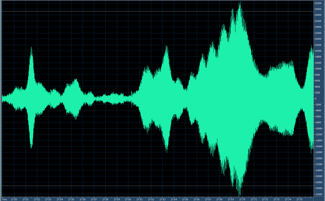
Figures 4 and 5, below, depict the rapid amplitude variations using a transmitted 4 kHz tone as an amplitude reference over a "Free Space Optical" path of approximately 15 miles (24km).  The horizontal axis is time and the vertical axis is linear amplitude.

Note the difference in horizontal time scales between the depictions, below:

Figure 4:
Scintillation of the laser-transmitted audio (4 kHz tone).
The time span of this particular graph is just over 250 milliseconds (1/4 second)
Click on the image for a larger version.

Figure 5:
Scintillation on the LED-transmitted audio (4 kHz tone).
In contrast to the image in Figure 4, the time span of this amplitude representation is nearly 10 times
greater - that is, approximately 2 seconds.  The rate and amplitude of the scintillation-caused
fading are dramatically reduced.
Click on the image for a larger version.

Laser scintillation:

As can be seen from Figure 4 there is significant scintillation that occurs at a very rapid rate.  The reference of this image is, like the others, based on a full-scale 16 bit sample.  Analysis of the original audio file reveals several things:

• While the "primary" period of scintillation is approximately 10 milliseconds (100Hz) but there is evidence that there are harmonics of this rate to at least 2.5 milliseconds (400 Hz) - but the limited temporal resolution of the test tone makes it difficult to resolve these faster rates.
• Other strong scintillatory periods evident in the audio sample occur at approximate subharmonics of the "primary" scintillatory rate, such as 75 and 150 milliseconds.
• The rate-of-change of amplitude during the scintillation is quite rapid:  Amplitude changes of over 30 dB (a factor of 1000) can occur in just 20 milliseconds.
• The overall depth of scintillation was noted to be over 40dB (a factor of 10000) with frequent excursions to this lower amplitude.  It was noted that this depth measurement was noise-limited owing to the finite signal-noise ratio of the received signal.

LED scintillation:

Figure 5 shows a typical example of scintillation from the LED using the same size emitter aperture as the laser.  Analysis of the original audio file shows several things:

• The 10 millisecond "primary" scintillatory period observed in the Laser signal is pretty much nonexistent while the 20 millisecond subharmonic is just noticeable.
  
• 150 and 300 millisecond periods seems to be dominant, with strong evidence of other periods in the 500 and 1000 millisecond range.
• The rate-of-change of amplitude is far slower:  Changes of more than 10 dB (a factor of 10) did not usually occur over a shorter period than about 60 milliseconds.
• The overall depth of scintillation was noted to be about 25 dB (a factor of about 300) peak, but was more typically in the 15-18dB (a factor of 32-63) area.

One of the more interesting results of this experiment was how minimally the severe amplitude distortion experienced with the laser actually degraded the overall intelligibility of human speech.  While the tones and brief music clips were clearly badly distorted, it could be argued that with the segment including speech, the degree of that distortion was not as apparent.  Clearly the voice content was being badly "chopped up" by the severe amplitude fluctuations, but with the redundant nature of speech and the fact that the drop-outs were quite brief in comparison to the duration of speech elements (sounds, syllables) it is quite reasonable to be able to expect the brain to fill in the gaps and make sense of it all.

A "Scintillation Compensator":

Despite the redundant nature of the speech maintaining reasonable intelligibility, it became quite "fatiguing" to listen to audio distorted in this manner so another device was wielded as part of an experiment:  The "Scintillation Compensator", the block diagram being depicted in Figure 6, below.

Figure 6:
Block diagram of the "Scintillation Compensator" system.
Click on the image for a larger version.

This system is essentially a "Keyed AGC" system using a low-level 4 kHz tone from the transmitter as an amplitude reference for a tracking gain cell at the receiver:  If the amplitude of the 4 kHz tone being received from the distant transmitter goes down, the gain of the audio in the receiver is increased by the same amount and vice-versa.  The effect of this device is quite dramatic as the clip in Figure 7, below, demonstrates:

Figure 7:

Audio clip with a"Before" and "After" demonstration

of the "Scintillation Compensator" 
Music:  "Children" by Robert Miles, used
in accordance with U.S. Fair Use laws.

One of the more striking differences is that in the "before" portion, the background hum from city lights remained constant while in the "after" portion it varied tremendously, more clearly demonstrating the degree of the amplitude variation being experienced.  What is also interesting is that the latter portion of the clip is much "easier" (e.g. less fatiguing) to listen to:  Even though syllables are lost in the noise, being obliterated by hum rather than silence in the first part of the above clip, the fact that there is something present during those brief interruptions, even though it is hum, seems to appease the brain slightly and maintain "auditory continuity".

It should be pointed out that the "Scintillation Compensator" cannot possibly recover the portions of the signals that are too weak (e.g. lost in the thermal noise and/or interference from urban lighting) but only that it maintains the recovered signal at a constant amplitude.  In the first portion of the clip in Figure 7 it was the desired signal level that changed while in the second portion it was the background noise that changed.  In other words, in both examples given in Figure 7, the instantaneous signal-to-noise ratio was the same in each case.

Practical uses for all of this stuff:

The most important point of this exercise was to demonstrate that a larger aperture reduces scintillation - although that point might be a bit obscured in the above discussion.  What was arguably more dramatic - and also important - was that the noncoherent light source seemed to be less susceptible to the vagaries of atmospheric disturbance.  This observation bears out similar testing done over the past several decades by many others, including Bell Labs and the works of Dr. Olga Korotkova.

For a brief bibliography and a more in-depth explanation of these effects visit the page "Modulated Light DX" - LINK - particularly the portion near the end of that page.

The reduction of scintillation has interesting implications when it comes to the ability to convey high-speed digital information across large distances using free-space optical means under typical atmospheric conditions.  Clearly, one of the more important requirements is that the signal level be maintained such that it is possible to recover information:  Too low a signal, it will literally be "lost in the noise" and be unrecoverable.

As the demonstrations above indicate, the "average" level may be adequate to maintain some degree of communications, but the rapid and brief decreases in absolute amplitude would punch "holes" in data being conveyed, regardless of the means of generating or detecting the light.  Combating this would imply the liberal use of techniques such as Forward Error Correction (FEC) and interleaving of data over time - not to mention some interactive means by which "fills" for the re-sending of missing data could be automatically requested.  The "'analog' analog" to these techniques is the aforementioned ability of the human brain to "fill in" and infer the missing bits of information.

While lasers are well-known to be "modulatable" at high rates, doing so for LEDs is a bit more problematic due to the much larger device (die) sizes and commensurate increase in device capacitance.  To rapidly modulate an LED at an ever-higher frequency would also imply an increase of "dV/dT" (e.g. rate of voltage change over time) which, given the capacitance of a particular device would also imply higher instantaneous currents within it, effectively reducing the average current that could be safely applied to it.  What this means is that it is likely that specialized configurations would required (e.g. drivers with fast rise-times at high current; structurally-small, high current/optical density LEDs etc.) to permit direct modulation of very high (10's of megabits) data rates.

Using the aforementioned techniques has rather limited utility when the free-space optical links extend out to many 10's of miles/kilometers owing largely to the vagaries of the atmosphere and the practical limits of optical flux with respect to "link margin" (e.g. the need to use safe and sane amounts of optical power to achieve adequate signal to recover information - particularly as the rate of transmission is increased) but it may be useful for experimentation.

Additional information on (more or less) related topics:

• Throwing One's Voice 95 miles on a lightbeam - link  - Details of experiments with high-power LEDs over a 95 mile (152km) optical path
• Voice on a Laser Beam - link - General information about using PWM techniques for Laser diode (and LED) modulation
• Gate Current in a JFET - link - The development of a highly-sensitive optical receiver that utilizes JFET gate current.
• The "Modulatedlight.org" web pages - link - This collection of web pages offers a large resource for many things related to free-space optical communications, including experiments, equipment and links to other related sites.
• For more information about the "Scintillation Compensator" and the "Audible S-Meter" used to set up the optical links, look at the page "An Audio Interface Device for Speech Bandwidth Optical Communications" - link

[End]

This page stolen from "ka7oei.blogspot.com".