A simple VHF notch cavity from scraps of (large) Heliax

In a previous post I discussed how a band-pass "cavity" could be constructed from a chunk of 1-5/8" Heliax ^(tm) cable (a link to that article is here).  This is the follow-up to that article.

Figure 1:
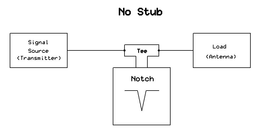
The dual notch filter assembly - installed at the
repeater.
Click on the image for a larger version.

Notch versus band-pass

As the name implies, a "notch" filter removes only a specific frequency, ideally leaving all others unaffected while a "band pass" filter does the opposite - it passes only a specific frequency.  Being the real world, neither type of filter is perfect - which is to say that the "width" of the effect of the notch or pass response is not infinitely narrow, nor is it perfectly inert at frequencies other than where it is supposed to work:  The notch filter will have some effect away from its frequency of rejection, and a band pass filter will let through off-frequency energy and both will have loss even where it would not be ideal.  These filters may be constructed many ways - from individual coils and capacitors to resonant structures, such as cavities - which are often larger-diameter tubes with smaller tubes inside, the latter being resonant at the frequency of interest.  The cavity-type of filters often have better performance as their operation is closer to that of ideal (perfect) components.

The degree to which a filters is imperfect is significantly determined by the "Q" (quality factor) of the resonating components and in general for a cavity-based device, the bigger the cavity (diameter of conductors and the container surrounding it) the better the performance will be in terms of efficacy - which is "narrowness" in the case of the notch filter and "width" and loss in the case of the band-pass cavity.

While a cavity-based device with a large inside resonator and larger outside container is preferred, one can use pieces of large coaxial cable, instead.  The use of large-ish coaxial cable as compared to smaller cable (like RG-8 or similar) is preferred as it will be "better" at everything that is important - but even a cavity constructed from 1-5/8" coax will be significantly inferior to that of a relatively small 4" (10cm) diameter commercial cavity - but there are many instance where "good" is "good enough.

Case study:  Removal of APRS/packet transmitter energy from a repeater input

As noted in the article about the band-pass cavities linked above, a typical repeater duplexer - even though it may have the words "band" and "pass" on the label and in the literature - RARELY have an actual, true "band-pass" response.  In other words, a true "bandpass" cavity/duplexer would have 10s of dB of attenuation, say, 20 MHz away from its tuned frequency - but most duplexers found on amateur repeaters will actually be down only 6-10 dB or so, meaning that even very far off-frequency signals (FM broadcast, services around 150-174 MHz, TV transmitters) will hit the receiver nearly unimpeded.  When I tell some repeater owners of this fact, I'm often met with skepticism ("The label says 'band-pass'!") but these days - with inexpensive NanoVNAs available for well under $100, they can check it for themselves - and likely be disappointed.

Many clubs have replaced their old Motorola, GE or RCA repeaters from the 70s and 80s with more modern amateur repeaters (I'm thinking of those made by Yaesu and Icom) and found that they were suddenly plagued with overload and IMD (intermod).  The reason for this is simple:  The old gear typically had rather tight helical resonator front-end filters while the modern gear is essentially a modified mobile rig - with a "wideband" receiver - in a box.  In this case, the only real "fix" would be the installation of band-pass cavities on the receive and transmit paths in addition to the existing duplexer.

In the case of APRS sharing a radio site, the problem is different:  Both are in the amateur band and it may be that even a "proper" pass cavity may not be enough to adequately reject the energy if the two frequencies are close to each other.  In this case, the scenario was about as good as it could be:  The repeater input was at 147.82 MHz - almost as far away as it could be from the 144.39 APRS frequency and still be in the amateur band.

What made this situation a bit more complicated was the fact that there was also a packet digipeater on 145.01 MHz - a bit closer to the repeater input,  but since it was about 600 kHz away from the 144.39 APRS frequency, that meant that just one notch wouldn't be quite enough to do the job:  We would need TWO.

Is it the receiver or transmitter?

Atop this was another issue:  Was it our receiver that was being desensed (overloaded) by these packet transmitters, or was it that these packet transmitters were generating broadband noise across the 2 meter band, effectively desensing the repeater's receiver?

We knew that the operators of the packet stations did not have any filtering on their own gear (the only way to address a transmit noise problem if generated by their gear) and were reluctant to spend the time, effort and money to install it unless they had compelling reason to do so.  Rather than just sit at a stalemate, we decided to do due diligence and install notch filtering on the receiver to answer this question - and give the operators of the packet gear a compelling reason to take action if it turned out that their transmitters were the culprit.

A simple notch cavity:

Suitable pass cavities are readily available for purchase new from a number of suppliers and used from auction sites - they are also pretty easy to make from copper and aluminum tubing - if you have the tools.  Because of the rather broad nature of a typical pass or lower-performance (e.g. broader) notch cavity, temperature stability is usually not much of an issue in that its peak could drift a hundred kHz and only affect the desired signal by a fraction of a dB.

As mentioned earlier, another material that could be used to make reasonable-performance pass cavities is larger-diameter hardline or "Heliax" ^(tm).  Ideally, something on the order of 1-5/8" or larger would be used owing to its relative stiffness and unloaded "Q" and either air or foam dielectric cable may be used, the main difference being that the "Q" of the foam cable will be slightly lower and the cavity itself will be somewhat shorter due to the different velocity factor.  If you have access to it and the appropriate machine tools there's no reason why similar devices might not be constructed using similar - or larger - sized copper or aluminum pipe.

Figure 2:
Cutting the (air core) cable to length
Refer to the calculator on the KF6YB web page, linked
at the end of this article.
Click on the image for a larger version.

The "Heliax notch cavity" described here can be built with simple hand tools, and it uses a NanoVNA for tuning and final adjustment.   While its performance will not be as good as a larger cavity, it will - in many cases - be enough to attenuate signals that are "far enough" away for the somewhat limited "Q" of a notch filter of this construction to be effective without excessively attenuating the desired frequency.

Using 1-5/8" "Heliax":

Note:  For an online calculator to help determine the length of cable to use, see the link to KF6YB's site at the end of this article.

The "cavity" described uses 1-5/8" air-core "Heliax" - and it is necessary for the inner conductor to be hollow to accommodate the coupling capacitors.  Most - but not all - cable of this size and larger has a hollow center conductor.  Cables larger diameter than 1-5/8" should work fine - and are preferred - but smaller than this may not or may note be practical in situations where the notch and desired frequency are closely spaced - this, for reasons of unloaded "Q".  If the center conductor is solid or if its inside diameter cannot accommodate the coupling capacitors (described later on) you will have to improvise their construction, using either a discrete variable capacitor or a small "sleeve" capacitor - external to the piece of cable similar to the coupling capacitors described below.

Preparing the "shorted" end:

For 2 meters, a piece of cable 18" long was cut.  For cables with an air dielectric, it's recommended that one cuts it gently with a hand saw rather than a power tool as the latter can "snag" and damage the center conductor.

Figure 3:
The "shorted" end of the stub with the slits bent to the middle
and soldered to the center conductor.
This end should be covered with electrical tape and/or
RTV/silicone to keep out insects/dirt.
Click on the image for a larger version.

For the "cold" (e.g. shorted) end, carefully (using leather gloves) remove about 3/4" (19mm) of the outer jacket and then clean the exposed copper shield with a wire brush, abrasive pad and/or sand paper.  With this done, use a pair of tin snips cut slots about 1/2" (12mm) deep and 1/4" (6mm) wide around the perimeter.  Once this is done, use a pair of needle nose pliers and remove every other tab, resulting is a "castellated" series of slots.  At this point, using a pair of diagonal pliers or a knife, cut away some of the inner plastic dielectric so that it is about 1/2" (12mm) away from the end of the center conductor.

Now, clean the center conductor so that it is nice and shiny and then bend the tabs that were cut inwards so that they touch the center conductor.  Using a powerful soldering iron (I used a 150 watter) or soldering gun - and, perhaps a bit of flux - solder the shield tabs to the center conductor all of the way around.  It's best to do this with the section of coax laying on its side so that hot solder/metal pieces do not end up inside the coax - particularly if air-core cable is used.  If you used acid-core flux, carefully clean it before proceeding.

With one end of the cable shorted you can trim back any protruding center conductor and file any sharp edges - again taking care to avoid getting bits of metal inside the air-space of the cable or embedded in the foam.  At some point, you should cover the shorted end with RTV (silicone) and/or good-quality electrical tape to prevent contamination by dust or insects.

Preparing the "business" end:

Figure 4:
This shows how the tube for the coupling capacitor is placed.
This photo is from the band-pass version with two tubes.
Click on the image for a larger version.

At this point, the chunk of coax should be trimmed again, measuring from the point where the center conductor is soldered to the shield:  For air-core trim it to 17" (432mm) exactly and for foam core, trim it to 16-1/8" (410mm).  Again, using a sharp knife and gloves, remove about 3/4" (19mm) of the outer jacket and, again, clean the outer conductor so that it is bright and shiny.

Making coupling capacitors:

We now need to make a capacitor to couple the energy from the coaxial cable to the center resonator and for this, we could use either a commercially-made variable capacitor (an air-type up to about 20pF - but much less will likely be required) or we could make our own capacitors:  I chose the latter.

At this point you may be asking yourself, "Self, if I make a coax stub for HF, I connect it directly to a coax Tee - why don't I do that here?"  While you could connect a 1/4" stub directly across the coaxial cable to effect attenuation, this is only practical for notches that are a significant distance away from the desired frequency.  For example, if you find yourself in the situation mentioned above (e.g. you replace your ancient repeater with a modern one with poor front-end filtering) where a nearby FM broadcast transmitter is overloading your receiver, you could reasonably measure/cut an open 1/4 wave stub for its frequency and put it across the coax feed with a "Tee" connector and reduce its energy by 20dB or so.  The problem is that a direct connection like this will have rather poor "Q" and be very wide - possibly suitable for a signal 10s of MHz away, but it won't help you if the signal is just a couple MHz away.

By "lightly" coupling to the resonator with a reactance - typically a capacitor in the 10s of pF range or lower - the "Q" of the resonating element is somewhat preserved and with "critical" coupling (not too much, not too little) one can achieve narrower, deeper notches.

Using RG-8 center for the coupling capacitor

For this, I cut a 3" (100mm) length of solid dielectric RG-8 coax, pulled out the center conductor and dielectric and threw the rest away.  I then fished around in my box of hardware and found a piece of hobby brass tubing into which the center of the RG-8 fit snugly cut to the same length as the center conductor.  If you wish, you can foam dielectric RG-8 center but be aware that it is more fragile - particularly when soldering.

I then soldered to tubing inside the center conductor/resonator as doing so offers good mechanical stability, preventing the piece of coax cable dielectric from moving around and changing its capacitance.

Using RG-6 center for the coupling capacitor:

While RG-8 and brass tubing is nice to use, I have also built these using the center of inexpensive RG-6 foam type "TV" coaxial cable and a small piece of soft copper water tubing that I had laying around - but it can easily be found at a hardware store.  This type of capacitor is fine for receive-only applications, but it is not recommended for more than a few watts:  The aforementioned RG-8 capacitor is better for that.

For this, I cut a 3" (75mm) long piece of RG-6 foam TV coaxial cable and from it, I removed and kept the center conductor and dielectric - removing any foil shield and then stripping about 1/2" (12mm) of foam from one end of each piece.

At this point, you'll need some small copper tubing:  I used some 1/4" O.D. soft-drawn "refrigerator" tubing, cutting a 2" (50mm) length and carefully straightening it out.  To cut this, I used a rotary pipe cutting tool which slightly swedged the ends - but this worked to advantage:  As necessary, I opened up the end cut with the deburring blade of the rotary cutting tool just enough that it allowed the inner dielectric of the RG-6 to slide in and out with a bit of friction to hold it in place.

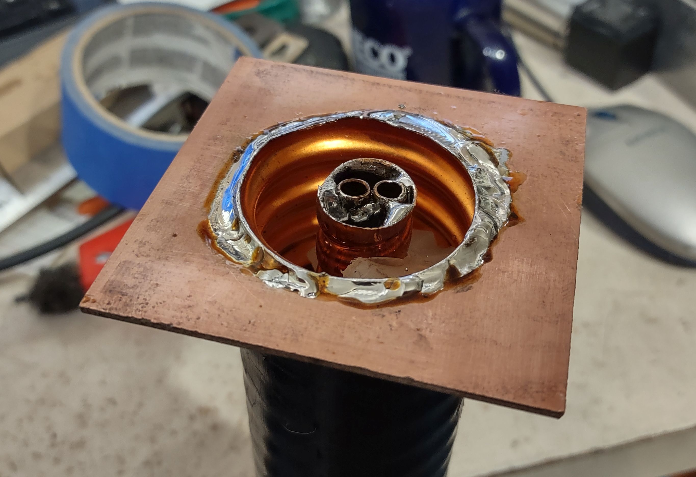
Figure 5:
The PC Board plate soldered to the end of the coax.  This
is from the band-pass version, but you get the idea!
Click on the image for a larger version.

No matter which type of coax center you are using, using a hot soldering iron or gun, solder the tube for the coupling capacitor inside the Heliax's center conductor, the end flush with the end of the center conductor:  A pair of sharp needle-nose pliers to hold it in place is helpful in this task.  Remember that you are soldering to a large chunk of copper, so you'll need a fair bit of heat to be able to make a proper connection!

Making a box:

On the "business" (non-shorted) end of the piece of cable we need to make a simple box with a solid electrical connection to the outer shield to which we can mount the RF connectors with good mechanical stability.  For the 1-5/8" cable, I cut a piece of 0.062" (1.58mm) thick double sided glass-epoxy circuit board material into a square that was 3" (75mm) square and using a ruler, drew lines on it from the opposite corners to form an "X" to find the center.

Using a drill press, I used a 1-3/4" (45mm) hole saw to cut a hole in the middle of this piece of circuit board material, using a sharp utility knife to de-burr the edges and to enlarge it slightly so that it would snugly fit over the outside of the cable shield:  You will want to carefully pick the size of hole saw to fit the cable that you use - and it's best that it be slightly undersized and enlarged with a blade or file than oversized and loose.

Figure 6:
Bottom side of the solder plate showing the
connection to the coax.
Click on the image for a larger version.

After cleaning the outside of the coaxial cable and both sides of the circuit board material, solder it to the (non-shorted) end on both sides of the board, almost flush with just enough of the shield protruding through the top to solder it.  For this, a bit of flux is recommended, using a high-power soldering iron or gun - and it's suggested that it first be "tacked" into place with small solder joints to make sure that it is positioned properly.

Adding sides and connectors:

With the base of the box in place, cut four sides, each being 1-3/8" (40mm) wide and two of them being 3" (75mm) long and the other two being 2-1/2" (64mm) long.  First, solder the two long pieces to the top, using the shorter pieces inside to space and center them - and then solder the shorter pieces, forming a five-sided (base plus four sides) box atop the piece of cable.

Figure 7:
A look inside the box showing the connection to the center of
the capacitor, the "tuning" strips and ceramic trimmer.
Click on the image for a larger version.

Resonator adjustment capacitor:

You will need to be able to make slight adjustments to the frequency of the center conductor of the Heliax resonator.  If all goes well, you will have cut the coaxial cable to be slightly short - meaning that it will resonate entirely above the 2 meter band.  The installation of the coupling capacitor will lower that frequency significantly - but it should still be above the frequency of interest so a means for "fine tuning" is necessary.

Figure 7 shows two strips of copper:  One soldered to the center conductor (the sleeve of the coupling capacitor, actually) and another soldered to the inside for the Heliax shield.  These to plates are then moved closer/farther away to effect fine-tuning:  Closer = lower frequency, farther = higher frequency.  Depending on how far you need to lower the frequency, you can make these "plates" larger or smaller - or if you can't quite get low enough in frequency with just one set of these "plates", you can install another set.  

NOTE:  It is recommended that you do NOT install the copper strips for tuning just yet:  Go through the steps below before doing so.

If your resonant frequency is too low - don't despair yet:  It's very likely that you'll have to reduce the coupling capacitor a bit (e.g. pull it out of the tubing and/or cut it a bit shorter) and this will raise the frequency as well.

How it's connected:

A single notch cavity is typically connected on a signal path using a "Tee" connector as can be seen in Figure 1:  At the notch's resonant frequency, the signal is literally "shorted out", causing attenuation.  

As can be seen in Figure 7, there is only one connector (BNC type) on our PC board box - but we could have easily installed two BNC connectors - in which case we would run a wire from one connector to the center capacitor as shown and then run another wire from the capacitor to the other connector.

Adjusting it all:

For this, I am presuming that you have a NanoVNA or similar piece of equipment:  Even the cheapest NanoVNA - calibrated according to the instructions - will be more than adequate in allowing proper adjustment and measurement of this device.

Using two cables and whatever adapters you need to get it done, put a "Tee" connector on the notch filter and connect Channel 0 on one side of the Tee and Channel 1 on the other side of the Tee and put your VNA in "through" mode.  (Comment:  There are many, many web pages and videos on how to use the NanoVNA, so I won't go through the exact procedure here.)

Configure the VNA to sweep from 10 MHz below to 10 MHz above the desired frequency and you should see the notch - hopefully near the intended frequency:  If you don't see the notch, expand the sweep farther and if you still don't see the notch, re-check connections and your construction.

At this point, "zoom in" on the notch so that you are sweeping, say, from 2 MHz below to 2 MHz above and carefully note the width and depth of the notch.  Now, pull out the center capacitor (the one made from the guts of RG-8 or RG-6 cable) a slight amount:  The resonant frequency will move UP when you do this.

The idea here is to reduce the coupling capacitance to the point where it is optimal:  If you started out with too much capacitance in the first place, the depth of the notch will be somewhat poor (20dB or so) and it will be wider than desirable.  As the capacitance is reduced, it should get both narrower and deeper.  At some point - if the coupling capacitance is reduced too much - the notch will no longer get narrower, but the depth will start to get shallower. 

Comment:  You may need to "zoom in" with the VNA (e.g. narrow the sweep) to properly measure the depth of the notch.  As the VNA samples only so many points, it may "miss" the true shape and depth of the notch as it gets narrower and narrower.

The "trick" with this step is to pull a bit of the coax center out of the coupling capacitor and check the measurement.  If you need to pull "too much" out (e.g. there's a loop forming where you have excess) then simply unsolder the piece, trim it by 1/4-1/2" (0.5-1cm), reinstall, and then continue on until you find the optimal coupling.

It's recommended that when you do approach the optimal coupling, be sure that you have a little bit of adjustment room - being able to push in/pull out a bit of the capacitor for subsequent fine tuning.

At this point your resonant (notch) frequency will hopefully be right at or higher than your target frequency:  If it is too low, you may need to figure out how to shorten the resonator a bit - something that is rather difficult to do.  If you already added the "capacitor plates" for fine-tuning as mentioned above, you may need to adjust them to reduce the capacitance between the ground and the center conductor and/or reduce their size.

Presuming that the frequency is too high (which is the desirable state) then you will probably need to add the copper capacitor strip plates as describe above, and seen in Figure 7.  You should be able to move the resonant frequency down toward your target by moving the plates together.  Remember:  It is the proximity of the plate connected to the center conductor of the resonator to the ground that is doing the tuning!  If you can't get the frequency low enough, you can add more strips to the center conductor - but you will probably want to remove the coupling capacitor (e.g. the coax center conductor) to prevent melting it when soldering.

Optimizing for "high" or "low" pass:

As described above, the notch will be more or less symmetrical - but in most cases you will want a bit of asymmetry - that is, you'll want the effect of the notch to diminish more on one side than the other.  Doing this allows you to place the notch frequency (the one to block) and the desired frequency (the one that you want) closer together without as much attenuation.

Figure 8:
The simplest form of the "high pass" notch, used during
initial testing of the concept - See the results in Figure 9.
Click on the image for a larger version.

"High-pass" = Parallel capacitor

In our case - with the higher of the two notches as 145.01 MHz and the desired signal at 147.82 MHz, we want the attenuation to be reduced rapidly above the notch frequency to avoid attenuating the 147.82 signal - and this may be done by putting a capacitor in parallel with the center of the coupling capacitor and ground:  A careful look at Figure 7 will reveal a small ceramic trimmer capacitor.

This configuration is more clearly seen in Figure 8:  There, we have the simplest - and kludgiest - possible form of the notch filter where you can see two ceramic trimmer capacitors connected across the center coupling capacitor and the center pin of the BNC connector.  Off the photo (to the upper-left) was the connection to a "tee" connector and the NanoVNA.  If you just want to get a "feel" for how the notch works and tunes, this mechanically simple set-up is fine - but it is far too fragile and unstable for "permanent" use.

For 2 meters, a capacitor that can be varied form 2-35pF or so is usually adequate - the higher the capacitance, the more effect there is on the asymmetry - but at some point (with too much capacitance) losses and filter "shape" will start to degrade - particularly with inexpensive ceramic and plastic trimmer capacitors.  Ideally, an air-type variable capacitor is used, but an inexpensive ceramic trimmer will suffice for receive-only applications - and if the separation is fairly wide, as is the case here.  For transmit applications, the air trimmer - or a high-quality porcelain type is recommended.

"Low-pass" = Parallel inductor

While the parallel capacitor will shift the shape of the notch's "shoulders" for "low notch/high pass" operation, the use of a parallel inductor will cause the response to become "low pass/high notch" where the reduced attenuation is below the notch frequency.  If we'd needed to construct a notch filter to keep the 147.22 repeater's transmit signal out of the 145.01 packet's receiver, we would use a parallel inductor.

It is fortunate that an inductor is trivial to construct and adjust.  For 2 meters, one would start out with 4-5 turns wound on a 3/8" (10mm) drill bit using solid-core wire of about any size that will hold its shape:  12-18 AWG (2-1mm diameter) copper wire will do.  Inductance can be reduced by stretching the coil of wire and/or reducing the number of turns.  As with the capacitor, this adjustment is iterative:  Reducing the inductance will make the asymmetry more pronounced and with lower inductance, the desired frequency and the notch frequency can be placed closer together - but decrease the inductance too much, loss will increase.

Comment:  The asymmetry of the "pass" and "notch" is why some of the common repeater duplexers have the word "pass" in their product description (e.g. "Band-Pass/Band-Reject"):  It simply means that on one side of the notch or the other the attenuation is lower to favor receive/transmit.  As noted later and seen in Figures 9 and 10, this "Band-Pass/Band-Reject" response does not indicate a significant amount of attenuation at frequencies far removed (by more than 5-10%) from the tuned frequencies.  If you are contemplating using devices with this sort of response at shared sites (e.g. other users) caution should be exercised in that interference to/from these other services may occur due to poor "off-frequency" filtering:  The addition of band-pass cavities is always recommended to prevent this.

Results:

Figure 9:
VNA sweep of one of the prototype notch filter depicted  in
Figure 8.  This shows the asymmetric nature of the notch and
"pass" response (blue trace) when a parallel capacitor is used.
 The yellow trace shows the low SWR at the pass frequency.
Click on the image for a larger version.

Figure 9 shows a the sweep of the assembly shown in Figure 8 from a NanoVNA screen.

The blue trace shows the attenuation plot:  At the depth of the notch (marker #1) we have over 24dB of attenuation, which is about what one can expect from a notch cavity simply "teed" into the NanoVNA's signal path.

We can also see the asymmetry of the blue trace:  Above the notch frequency we see Marker #2 - which is a few MHz above the notch and how the attenuation decreases rapidly - to less than 0.5dB.  In comparison the blue trace below the notch frequency has higher attenuation near the notch frequency.

If you look carefully you'll also notice that just above the notch frequency, the attenuation (blue trace) is reduced to the lowest value right at the desired pass frequency:  This is our goal - set the notch at the frequency we want to reject and then set the parallel inductor or capacitor to the value that yields the lowest attenuation and lowest VSWR (the yellow trace) at the frequency that we want to pass.

Again, if we'd placed an inductor across the circuit rather than a capacitor, this asymmetry would be reversed and we'd have the lower attenuation below the notch frequency.

Note:  This sweep was done with the configuration depicted in Figure 8 at whatever frequency it happened to resonate "near-ish" 2 meters to test how well everything would work.  Once I was satisfied that this notch filter could be useful, I rebuilt it into the more permanent configuration and tuned it properly, onto frequency.

Putting two notches together:

Because we needed to knock down both 144.39 and 145.01 MHz, we can see from the Figure 9 that we'd need two notch filters cascaded to provide good attenuation and not affect the 147.82 MHz repeater input frequency.  A close look at Figure 1 will reveal that these two filters are, in fact, cascaded - the signal from the antenna (via the receiver branch of the repeater's duplexer) coming in via one of the BNC Tees and going out to the receiver via another.

The cable between the two notches should be an electrical quarter wavelength - or an odd multiple thereof (e.g. 3/4, 5/4) to maximize the effectiveness of the two notches together:  Since we only need a very short cable, we can use 1/4 wavelength here.  A quarter wave transmission line has an interesting property:  Short out one end and the impedance on the other end goes very high - and vice-versa.  To calculate the length of a quarter-wave line we can use some familiar formulas:

300/Frequency (in MHz) = Wavelength in meters

If we plug 145 MHz into the above equation (300/145) we get a length of 2.069 meters (multiply this by 3.28 and we get 6.79 feet).

Since we are using coaxial cable, we need to include its velocity factor.  Since the 1/4 wave jumper is foam-type RG-8X we know that its velocity factor is 0.79 - that is, the RF travels 79% of the speed of light through the cable, meaning that it should be shorter than a wavelength in free space, so:

2.069 * 0.79 = 1.63 meters (5.35')

(Solid dielectric cable - like many types of RG-8 and RG-58 will have a velocity factor of about 0.66, making a 1/4 wave even shorter!  There are online tables showing the velocity factor of many types of cable - refer to one of these if you aren't sure of the velocity factor of your cable.)

Since this is a full wavelength, we divide this length by 4 to get the electrical quarter-wavelength:

1.63 / 4 = 0.408 meters (16.09")

As it turns out, the velocity factor of common coaxial cables can vary by several percent - but the length of a quarter-wave section is pretty forgiving:  It can be as much as 20% off in either direction without causing too much degradation from the ideal (e.g. it will work "Ok") - but it's good to be as precise as possible.  When determining the length of the 1/4 wave jumper, one should include the length to the tips of the connectors, not just the length of the cable itself. 

Figure 10:
The response of the two cascaded notch filters - one tune to
144.39 and the other to 145.01 MHz.
Click on the image for a larger version.

Because we know that the notch filters present a "short" at their tuned frequency, that means that the other end of a 1/4 wave coax at that same point will go high impedance - making the "shorting" of the second cavity even more effective.  In testing - with the two notches tuned to the same frequency, the total depth of the notch was on the order of 60dB - significantly higher than the sum of the two notches individually - their efficacy improved by the 1/4 wave cable between them.

As we needed to "stagger" the two notches to offer best attenuation at the two packet frequencies, the maximum depth was reduced, but as can be seen in Figure 10, the result is quite good:  Markers 1 and 2 show 144.39 and 145.01 MHz, respectively with more than 34 dB of attenuation:  The two notches are close enough to each other than there is some added depth by their interaction.  Marker 3 at the repeater input frequency of 147.82 has an attenuation of just 0.79dB - not to bad for a homebrew filter made from scrap pieces!

Comment:  If you are wondering of the 0.79dB attenuation was excessive, consider the following:  Many repeaters are at shared sites with other users and equipment - in this case, there were two other land-mobile sites very nearby along with a very large cell site.  Because of this, there is excess background noise generated by this other gear that is out of control of the amateur repeater operator - but this also means that the ultimate sensitivity is somewhat limited by this noise floor.  Using an "Iso-Tee", it was determined that the sensitivity of this repeater - even with coax, duplexer and now notch filter losses - was "site noise floor limited" by a couple of dB, so the addition of this filter did not have any effect on its actual sensitivity.

Putting it together:

Looking again at Figure 1, you will noticed that the two notches filters are connected together mechanically:  Short pieces of PVC "wood" (available from the hardware store) were cut and a hole saw was used to make two holes in each piece, slipped over the end and then secured to the notch assemblies with RTV ("Silicone") adhesive.

Rather than leaving the tops of the PC board boxes open where bugs and debris might cause detuning, they were covered with aluminum furnace tape which worked just as well as soldering a metal lid would have - plus it was cheap and easy!  (The boxes were deep enough that the proximity of metal - or not - at the top had negligible effect on the tuning of the resonators.

Did it work?

At the time we installed the filter, the packet stations were down, so we tested the efficacy of the filter by transmitting at high power on the two frequencies alternately from an on-site mobile-mounted transceiver.  Without the filter, a bit of desense from this (very) nearby transmitter was noted in the receiver, but was absent with it inline.

With at least 34dB of attenuation at either packet frequency we were confident that the modest amount of desense (on the order of 10-15dB - enough to mask weak signals, but not strong ones) - IF it was caused by receiver overload - would be completely solved by attenuating those signals by a factor of over 2000.  If it had no effect at all, we would know that it was, in fact, the packet transmitters generating noise.

Some time later the packet stations were again active - but causing a bit of desense, but this was not unexpected:  At the start, we were not sure if the cause of the desense was due to the repeater's receiver being overloaded, or noise from the packet transmitter - but because the amount of desense was the same after adding the notch filter we can conclude that the source of desense was, in fact, noise from the packet transmitters.

Having done due diligence and installed these filters on our receiver, we could then report back to the owner of the packet transmitters what we had done and more authoritatively request that they install appropriate filtering on their transmitters (notch or pass cavities - preferably the latter) in order to be good neighbors, themselves.

* * *

"I have 'xxx' type of cable - will it work?"

The dimensions given in this article are approximate, but should be "close-ish" for most types of air and foam dielectric cable.  While I have not constructed a band-pass filter with much smaller Heliax-like cable such as 1/2" or 3/4", it should work - but one should expect somewhat lower performance (e.g. not-as-narrow band-pass with higher losses) - but it may still be useful.  With these smaller cables you may not be able to put the coupling inside the center conductor, so you'll have to get creative.

Because of the wide availability of tools like the NanoVNA, constructing this sort of device is made much easier and allows one to characterize both its insertion loss and response as well as experimentally determining what is required to use whatever large-ish coaxial cable that you might have on-hand.

"Will this work on (some other band)?"

Yes, it should:  Notch-only filters of this type were constructed for a 6 meter repeater - and depending on your motivation, one could also build such things for 10 meters or even the HF bands!

It is likely that, with due care, that one could use these same techniques on the 222 MHz and 70cm bands provided that one keeps in mind their practical limitations.

 

 * * *

Related articles:

• A 2-meter band-pass cavity using surplus Heliax - link - This article describes constructing a simple band-pass filter using 1-5/8" Heliax. The techniques used in that article are the same as those applied here.
  

• Second Generation Six-Meter Heliax Duplexer by KF6YB - link  - This article describes a notch type duplexer rather than pass cavities, but the concerns and construction techniques are similar.
  

• When Band-Pass/Band-Reject (Bp/Br) Duplexers really aren't bandpass - link - This is a longer, more in-depth discussion about the issues with such devices and why pass cavities should be important components in any repeater system.

 

* * *

This page stolen from ka7oei.blogspot.com

[End]

Revisiting the 20 meter "helical resonator" band-pass/notch filters

In my June 30, 2014 blog entry (linked here) I described simple band-pass and band-stop filters that could offer a degree of isolation between two 20 meter stations.

Why is this important?  Having more than one station on, say, 20 meters is advantageous because (with Field Day, at least) a separate 20 meter SSB and a 20 meter CW (or digital) station will count as two stations on separate "bands".  Having two transmitters on the same amateur band, in close proximity, offers a significant challenge - requiring as much antenna separation as possible and the careful selection radios that will "play nice" in the presence of each other.

These filters would be unique compared other "HF band" filters (e.g. "Dunestar" or any other filter that is designed to work on a specific band) in that not only would they be offer some rejection from another station on the same band, but you would also be able to transmit through it with acceptable losses.

An added challenge is that some modern software-defined radios use "direct sampling" RF front ends and these are arguably less-able to deal with very strong, nearby transmitters than their analog counterparts - particularly if the other transmitter is operating on a frequency within its band-pass filtering:  In other words, with a radio like an Icom IC-7300, you probably can't co-exist with another station on the same band - Even the "Digi-Sel" in your IC-7610 might not be able to save you!

* * *

As a bit of a challenge to myself, I decided to make these filter elements as cheap as possible, choosing to construct them to fit within a metal 1 gallon paint can.  As noted in the article linked above, the volume of these cans are actually slightly too small for optimal use at 20 meters, but I decided to see what I could do.

Details of the construction of these filters is described in the article linked above.  I will reiterate:  There are certainly better ways to implement many of the aspects of these filters than the way that I did it - but it is a starting point, if nothing else.

How they are used:

Figure 1:
The 20 meter notch (left) and band-pass filters.  These filters, constructed
using gallon paint cans, can be used to provide a degree of isolation between
two stations operating on the 20 meter band - such as an SSB and a
CW/digital station.
Click on the image for a larger version.

The idea is simple - with two separate components:

• A band-pass filter for use on the CW (or digital) station that would pass the (comparatively) narrow range of frequencies likely to be used for operation in that narrow portion of the 20 meter amateur band.  These would be tuned to pass energy in the general area of 14.02 to 14.08 MHz.

• A band-stop (a.k.a. "notch") filter that would be used on the SSB station to reduce the amount of impinging energy from the CW (or digital) station, tuned to the same frequency range as being used for transmitting by that station.

The above strategy can work because the CW (or digital) station will operate over a rather narrow frequency range - a few 10s of kHz at most - which means that retuning is not required for the notch filter used on the SSB station and only minor "touch up" tuning might ever be required for the CW/digital station.

When I originally constructed these filters I had available a few pieces of test equipment:

• Signal generator/transmitter
• Power meter/watt meter
• A broadband noise generator
• A calibrated spectrum analyzer

For measuring insertion loss and checking general matching, one's own HF transciever along with a dummy load and wattmeter is more than adequate:  It will give a real-world indication of the insertion loss of the filter - and a VSWR meter will provide a general indication of the state of the match at the various frequencies.  If the radio being used has a built-in antenna tuner, slight mismatching cause by the filter may be "removed" from the point of view of the radio to assure maximum power transmission through the device.

For determining the rejection of the notch or loss of the band-pass filter the task is a bit trickier, so I used what was available:  A broad-band noise source and a spectrum analyzer - this combination being used in lieu of a spectrum analyzer with a tracking generator.  Practically speaking, the use of a tracking generator versus a noise source amounts to different measurement techniques as they can, in this instance, give equivalent results - but a detailed discussion of this could be the entire topic of a different article!

Re-testing the "paint can" filters with a VNA:

I recently added another piece of equipment to my workbench:  A DG6SAQ "VNWA" (read about that device here - sdr-kits.com).  This is a reasonably-priced (in the $550-$700 range, depending on options, exchange rates, etc.) piece of equipment, usable from a few kHz up to about 1.3 GHz, that can do a "proper" job of analyzing an RF device, being able to measure insertion loss, return loss (which can be used to calculate VSWR) and complex impedance - just to name a few.  For the purposes of building, testing and analyzing RF filter circuits like this - and RF amplifiers - it is a more useful tool than a spectrum analyzer+tracking generator.

Comment:

The ubiquitous "NanoVNA" has appeared on the scene since this article was originally written.  When properly calibrated, even the least expensive of these will do a very good job in terms of measurement of their properties and allow careful and accurate adjustment.

While the equipment originally used (transmitter, wattmeter, analyzer) can be used to analyze the critical properties of the filter, the use of a Vector Network Analyzer can simultaneously give several parameters about the nature of the filters' parameters.  It should go without saying that this allows comparatively easy tweaking of the tuning and coupling of the resonators - as well as trying different configurations - and observing the results real-time.

Bandpass filter analysis:

Armed with this gear, I set the bandpass resonator on the workbench and used the VNA to measure its properties.

Figure 2:
VNA plots of the 20 meter helical bandpass filter showing the insertion loss (the blue line near the top) and the impedance (the red circle overlaying the series of green circles) at at various frequencies.
Click on the image for a larger version.

As can be seen, the insertion loss points are as follows:

• 14.07 MHz:  1.3dB.  At this frequency the match is quite good - well inside the inner-most green circle, which denotes a VSWR of 1.5:1 or better.
• 14.15 MHz:  3dB
• 14.25 MHz:  >6dB
• 14.35 MHz:  9dB

These figures aren't spectacular when it comes to off-frequency rejection and this is pretty much a limit of the loaded "Q" of the filter.  Unfortunately, there isn't too much that can be done about this without dramatically changing the physical design of the bandpass filter - notably decreasing the losses associated with the resonating inductor, but aside from silver-plating it (which would help only "somewhat") it would take some combination of a conductor with much larger surface area and the use of a larger enclosure - or adding a second such filter in series with the first.

(At this time, I do not have a second band-pass filter on-hand or else I would have done an analysis with two connected in series.)

Having said this, reducing the power of an offending signal by just 6 dB (e.g. the attenuation at 14.25 MHz when the peak is set to 14.07 MHz) can have a significant effect on the reduction of the symptoms of front-end overload - particularly if one ascribes the idea that a 6 dB reduction correlates to a 18 dB reduction of intermodulation products according to the "1:3" IMD rule in this situation.


Out-of-band rejection of the 20 meter band-pass filter:

Knowing the efficacy of a single bandpass filter element within the 20 meter band, the question arose:  How well does this filter remove out-of-band frequencies?  The VNA provided an easy answer:

Figure 3:
Plot showing attenuation on the 40, 30, 17, 15, 12 and 10 meter amateur bands through the single 20 meter resonator.  The attenuation figures for various bands can be read in the upper left-hand corner of the plot.
Click on the image for a larger version.

Looking at Figure 3 we note that on the bands below 20 meters, the single band-pass filter has excellent rejection - exceeding 39 dB on 30 meters and over 50 dB on 40 meters and below.  As expected with a capacitively-coupled resonator, the attenuation above the design frequency isn't as good, but it exceeds 25 dB on all HF bands.  By itself, this filter would do an excellent job in reducing overload from adjacent-band signals - particularly on bands lower than 20 meters.

Band-stop (notch) filter analysis:

With a UHF "tee" connector right at the notch resonator (connected as depicted in Figure 5) one gets the results shown in Figure 4, below:

Figure 4:
The "notch" response with no stub between the Tee and the notch resonator.
Click on the image for a larger version.

As seen in Figure 4, the notch has relatively little effect in the upper end of the band (above about 14.2 MHz) - which is as it should be - but the notch depth is only around 6 dB in the CW/digital segment - again, a result of the resonator's limited "Q" and other factors that reduce it from the ideal.

Figure 5:
Notch with no "stub" - the result being shown in the plot
of Figure 4, above.
Click on the image for a larger version.

Fortunately, there's something that we can do about this:  Change the impedance at the resonator in our favor.

If one takes a look at the red circle, we can see that the resistance at marker #1 is in the area of 15 ohms.  If we apply a length of transmission line, we can use it to transform the impedance at the "Tee" connector to do a better job of shunting RF at a particular frequency.

Here's what happens if a 1/4 wavelength stub is connected between the "Tee" and the notch filter, connected in the manner depicted in Figure 7:

Figure 6:
The "notch" with a 1/4 wavelength stub inserted between the Tee and the resonator.  As we can see, the notch depth is greatly increased - around 25dB - but the response isn't particularly useful!
Click on the image for a larger version.

Adding the 1/4 wavelength stub of RG-8 type cable greatly increased the notch depth - around 25dB - and this is evidenced by the fact that the red marker (#4) shows, in the circle, an impedance of just a few ohms.  Unfortunately, this has two undesired effects:

Figure 7:
A stub between the tee and notch element.  As can be seen
in Figures 6 and 7, the length of this stub can change
the depth of the notch and the "shape" of the notch and
the attenuation of the nearby frequencies that are not
to be notched out.
Click on the image for a larger version.

• The frequency "distance" between the notch and the peak is now too wide - greater than the width of the 20 meter band.  This means that this configuration is not really usable for our intended purpose.
• There is now an asymmetry in the response:  The "peak" (minimum attenuation) is lower in frequency than the notch.

Also note that an upward frequency shift of the notch occurred due to various factors - mostly the reduced "loading" of the resonator - but because I was interested in the shape of the response rather than the actual frequency,  I did not retune the notch to the target frequency.

What about using something shorter than a 1/4 wave to do a less-dramatic transformation?

Figure 8:
The same arrangement as in Figure 4, but with a shorter cable - one that is approximately 0.15 wavelength.  The VSWR is acceptable with radios with built-in tuners - but careful adjustment of coupling and stub length could bring more of the red circle to the 50 ohm "center" of the green circles of the Smith plot.
Click on the image for a larger version.

In figure 8, a shorter cable was used - one that was about 0.15 wavelength of RG-8 type cable.  As figure 8 shows, the attenuation isn't as great - around 10 dB - but we we see that there is minimal effect on frequencies above 14.2 MHz and we see something else that is interesting:  An asymmetrical response that works in our favor:  There is less attenuation above the notch - where our SSB operation is to occur - than below it.  This "trick" is frequently used in notch filters - such as those used for repeater duplexers - to increase both the notch depth and provide an asymmetry that favors the frequency at which one wishes to have the least amount of attenuation, typically done with the use of parallel (shunt) capacitance and inductance - both being things that I have yet to try with these filters.

Its worth noting that even though there was a frequency shift with this stub, it was much less than that depicted in Figure 6, so I was able to easily re-tune it.

Two notch filters cascaded:

As it happens, I do have two devices that may be used as a notch resonator - the second one being the band-pass resonator - if I use only one of its ports.  The results are as follows:

Figure 9:
The result of cascading two notch filters.  The insertion loss is only slightly higher, but the notch depth is now over 20dB.
In reality, the second "notch" filter was just the band-pass filter with only one of the two ports connected.  A bit more tweaking would likely have reduced the insertion loss and brought the "pass" frequencies' matches closer to 50 ohms.
Click on the image for a larger version.

In this test I placed two notch filters in succession as depicted in Figure 10 - using 0.15 wavelength stubs between the two "tee" connectors (and notch resonators) and between the tees and the resonators themselves:  For some reason, I seem to have a bunch of RG-8 jumpers of about that length - around 0.15 wavelengths at 20 meters, which works out to be in the area of 7-8 feet (a bit over 2 meters) physical length, so that is what I used.

Figure 10:
Two notch elements connected with stubs to improve performance.
With properly selection of stub length, not only can the notch depth be "greater than the sum of the parts", but the actual shape of the response can be adjusted.  For Figure 9, all of the stubs had an electrical length of approximately 0.15 wavelength - but no additional testing was done with other lengths at this time.
Click on the image for a larger version.

As Figure 9 shows, the notch depth is a bit over 20 dB and there is only a slight increase in insertion loss to the 20 meter SSB frequencies:  Clearly, this configuration is definitely having a significant effect on the undesired CW/SSB signal and would probably solve most in-band overload issues!

Final comments:

No doubt different (better!) results could have been obtained with different stub lengths and configurations along with the use of parallel (shunt) capacitance and inductance to produce an asymmetrical  responce, but I have only so much time and not all that many random chunks of cable on hand and, more importantly, until(?) I construct another notch and pass resonator, I won't be able to use two cavities in the field.

One thing that is difficult to predict before-hand is the effect of source and load impedances other than ideal 50 ohm resistive that would be present with the output (transmit) and input (receive) impedances of HF transceivers, which are "nominally" 50 ohms:  In reality, these impedances can vary quite a bit (even between receive and transmit on the same radio!) and these differences can have an effect on the precise amount of attenuation that will be seen.  Practically speaking, it will be the transmit loss that will be considered - and this will also be affected by the radio's built-in antenna tuner, if it is inline.  Yet another factor that will affect the performance is the match of the connected antenna - particularly as seen at the far ("radio") end of the feedline - especially if a tuner is used there, too.

* * *

What would I do different if I construct more of these things?  As noted in the original June 30, 2014 blog entry (linked here) a major weak point of these resonators is the physical construction of the capacitive coupling probes:  They are not easy to adjust, and they are quite fragile - a good "jar" of the filter (pun intended!) can knock things out of position and cause detuning.  Having a means of being able to adjust the coupling without disassembly - perhaps the use of plastic screws accessible from outside the filter - would be very useful, allowing both critical coupling and tuning to be better-achieved while greatly improving ruggedness.

Perhaps, that will be a future project.

* * *

This page stolen from ka7oei.blogspot.com

[End]
 

Managing HF signal dynamics and preventing overload with the RTL-SDR (and KiwiSDR) receivers

Note:  This article was inadvertently posted for a few days before it had been finished.  This is the "completed" version of that article.

The Kiwi SDR:

The Kiwi SDR is a stand-alone network-connected multi-user "SDR in a box" device with its own web interface that allows one to tune from (nearly) DC to at least 30 MHz.  Using a 14 bit A/D converter, it is more robust than the RTL-SDR mentioned below, but it can still be overloaded by strong AM broadcast stations - so what follows can be applied.

The "RTL-SDR":

The so-called "RTL-SDR" dongles are devices that have become quite popular owing to their low cost (anywhere between $10 and $100, depending on features) and their ability to cover a wide frequency range - typically from a few hundred kHz to nearly 1GHz, depending on the device.  There are two separate signal paths on these devices:

• Via the Raphael R820 chip.  This has an onboard synthesizer, mixer and band-pass filters and it converts signals in the (approximately) 24-1300 MHz range to a lower frequency.  This is the "normal" signal path used in these RTL-SDR dongles when used as they were originally designed for reception in the VHF and UHF bands.
• Direct, into the RTL2832 chip.  This (typically unused) input may be made available via another connector, or via a frequency-splitting filter network as is done on the "RTL-SDR Blog" dongles.  This input can work from a few 100 kHz to 10s of MHz, more or less in conjunction with this chip's tuner/synthesizer.

It is the RTL2832 that has the A/D converter - which is just 8 bits - and that is the main limit of these devices when used in environments with both strong and weak signals.

Receiving HF with an RTL-SDR dongle:

If we want to receive the HF spectrum - which we'll call 500kHz-30 MHz (we'll include MF here...) we have to work around some issues.  The most obvious is that the R820 chip can typically tune down to something in the 20 MHz range (it can sometimes be coaxed to go even lower) but it certainly cannot be relied on to work well in the 1-5 MHz range.

The "direct" input has the advantage that is uses an 8-bit A/D that is sampling at 28.8 MHz followed by some DSP logic that allows signals in that stream to be internally converted to "baseband" samples - but the nature this chip poses a few problems.  To receive the entire HF spectrum, we have two methods that may be used, but each of these has their own sets of quirks, advantages and disadvantages:

The "direct" method:

• It is very simple to implement in that it uses would would normally be an unused input.  Many dongles already include this modification - but if not, it may be easily added (instructions may be found on the web.)
• The frequency stability can be better than the "upconversion" method since it is always lower - and there is only one oscillator that must be kept stable.
• This has the disadvantage that the sample rate is about 28.8 MHz meaning that signals above 14.4 MHz will be aliased.  For example, a signal at 21.25 MHz will also appear at (28.8 - 14.4 = ) 7.55 MHz.  This can usually be mitigated by the addition of band-pass filtering around the frequencies of interest if "fixed frequency" operation is expected.
• The "direct" input is typically quite "deaf", often requiring a bit of amplification if it is to be used for microvolt-level signals.  In testing, it took about 7 microvolts (-90dBm) for a CW signal to become audible, about 15 microvolts (-84dBm) for an SSB signal to be readable and around 25 microvolts (-79 dBm) for an AM signal to become listenable.  In other words, the sensitivity of this unit in direct mode is 20-30dB worse than a modern receiver.  The RTL-SDR dongles used happen to have a built-in amplifier so their sensitivity is "reasonable".

The "up-converter" method: 

• In this method there are two oscillators that can contribute to drift:  The (typically) 100 or 125  MHz oscillator used for the up-conversion and the clock reference in the receiver itself.  Because both of these oscillators are operating at a rather high frequency - and because there are two of them - drift can be exacerbated.
• The "image" problem associated with "direct" method is largely avoided.
• The mixers used for frequency conversion can, in some cases, be overloaded by strong signals meaning that signals may be degraded before they get to the receiver.

No matter the configuration, there is one limitation intrinsic to these "RTL" devices:  The 8 bits of A/D conversion.

The "dynamic range" problem:

With 8 bits one can only attain an overall dynamic range of about 48dB (the actual amount is actually harder to calculate owing to oversampling, thermal and circuit noise, external noise, etc.)  The problem arises from the fact that a "weak" signal at, say, 160 meters may be on the order of 1 microvolt (-107dBm) but a nearby AM broadcast transmitter may be presenting a signal that could be 500 microvolts (-53dBm) or even much more!  In our example, we can see that this could pose a signal difference of 54dB - greater than the range that can be represented using an 8 bit converter.  In other words, assuming a 48dB dynamic range of our A/D converter, if we adjusted our levels so that a 1 microvolt signal (-107dBm) just barely registered on the A/D, any signal(s) that were 48dB above this (-59dBm) would "max out" our converter - again, ignoring oversampling, etc.

In other words, if we were to carefully adjust our signal level to our RTL-SDR (using an attenuator) such that we were just below the signal level that "maxed out" our A/D converter, our weak signal would be below the signal level represented by the lowest bit and it would (probably) be lost in the noise.  Conversely, if we tried to bring the weak signal up to the point where it was out of the quantization noise of the A/D converter, we'd be overloading our A/D, causing distortion and making it work very badly.

The importance of band-pass filters:

Whether you are using the RTL-SDR dongle in the "direct" mode with with a converter it would be a very good idea to limit the signals arriving at its input to only those of interest as much as possible.  This need contradicts the desire of many users of this device to cover from "DC to Daylight" - but if one attempts to put such a large frequency range into the antenna, performance will suffer imensely:  If the unit doesn't just overload, there will likely be issues with trying to receive weak signals in the presence of strong ones - and with just 8 bits of A/D conversion, if that difference is greater than 40dB, you may see significant degradation.

When used in the "normal" mode where the R820 chip is acting as frequency converter, the A/D converter in the RTL2832 chip sees a somewhat limited spectrum owing to filtering in the R820 chip - but despite this filtering there is still the problem of "weak versus strong" signals that are within this passband - not to mention the fact that it just doesn't take a lot of signal to overload the R820 outright.

If you are using "Direct sampling" mode on HF, the program is more severe:  The entire HF spectrum being applied at the RF input is being digitized by a measly 8 bits which means that even if you are running the RTL2832 in the 2048ksps mode where you can "see" 2 MHz of spectrum, signals from the rest of the spectrum are still being digitized by that 8 bit converter.  If you consider that the signal-handling capability of the 8 bit A/D to be a limit to the total RF power being applied, you may be "wasting" much of this A/D capability at frequencies that are of no interest to you at all!

Images in the "direct" mode:

A worst-case example:  20 meters

If you are running "direct" mode, the problem is worse, still:  As noted above, the sampling rate of the A/D converter is 28.8 MHz, which means that signals above the Nyquist limit at half this frequency - 14.4 MHz - will "reappear" elsewhere.  For example, if you were listening at 14.300 MHz on the 20 meter band - which is 100 kHz below the 14.4 Nyquist limit - you would also hear signals at 14.500, which is 100 kHz above the Nyquist limit.  Similarly, if you were tuned to an AM broadcast station at 1.0 MHz - 13.4 MHz below the Nyquist limit - you would hear signals that were at 27.8 MHz - 13.4 MHz above the Nyquist limit.

In the second case it's pretty easy to filter out the 27.8 MHz signals:  A simple low-pass filter will do, but in the first case - using the RTL-SDR Dongle at 20 meters - things are quit different as it is difficult to build a filter that will pass signals at 14.35 MHz with little attenuation but block signals at 14.45 MHz - the "image" of 14.35 MHz - sufficiently.  What this means is that if you are several MHz away from this 14.4 MHz limit, you can probably get away with filtering in the "direct" mode - but the closer you get (say, within the 13-16 MHz range) the more difficult it will be to remove the image.

The typical work-around for this is to convert the HF range to a higher frequency - typically by mixing it with a local 125 MHz oscillator, so instead of 20 meters being tuned in at 14.0-14.35 MHz in direct mode, it would be at 139.0-139.35 MHz.  This works pretty well, although oscillator stability - both in the RTL-SDR dongle's synthesizer and in that added 125 MHz oscillator - is much more of a concern as the frequency at this 139 MHz frequency could drift hundreds of Hz between the two oscillators whereas in direct mode - with only one oscillator - the absolute frequency is much lower (about 1/10th) along with the amount of drift.

Even with the "upconverting" technique, you are not excused from needing to have front-end filtering:  The limits of the 8 bits of A/D conversion and those of the circuitry still apply!

Another approach for 20 meter coverage:

Taking our 20 meter example, while we could upconvert - which would be the easiest approach if  you happened to buy an RTL-SDR with an upconverter - another approach would be to convert the frequency band from 14.0-14.35 MHz down to, say, 4.0-4.35 MHz by using a mixer and a 10 MHz oscillator:  This lower frequency would imply higher stability and the filtering requirements would be greatly relaxed as compared to up-converting by 100 or 125 MHz:  An example of such a circuit may be seen below in Figure 1.

Figure 1:
20 meter converter for an RTL-SDR Dongle used in "direct" mode.  This mixes the incoming (filtered) 20 meter signals with 10 MHz to produce a 4.0-4.35 MHz output.  Originally, I'd planned to use an inexpensive 10 MHz TCXO, but it was unavailable at the time of construction.  In the upper-right corner is an representation of the circuit layout.
Click on the image for a larger version.

In the diagram above we see the signals coming in and being applied to a 2-pole bandpass filter for 20 meters.  I "borrowed" this design from QRL Labs' bandpass filter (link) - so if you don't wish to build your own, you may order a kit of parts for the band of your choice from them.

This filter is not nearly "sharp" enough to pass the top end of the 20 meter band (14.35 MHz) and sufficiently block its nearest image frequency (14.45 MHz) if we were to use "direct" mode with the 14.4 MHz Nyquist limit so we down-convert the 20 meter band from 14.0-14.35 to 4.0-4.535 MHz, instead - well away from from the image response.  The bandpass filter limits the number of signals that get converted and provide enough filtering to minimize an image response that could occur due to the converter itself - that of the sum frequency (e.g. 24.0-24.35 MHz).  Transistor Q1 boosts the HF signal somewhat to overcome the loss of the filter and of the mixer and low-pass filter following it.

The local oscillator that I used was a 10 MHz OCXO (Oven-controlled Crystal Oscillator) that I had kicking around and its output was at TTL levels - a 5 volt square wave, so R5 was placed in series to knock this down to about 1 volt peak-peak at the "LO" input of U1, a diode-ring mixer.  I had originally intended to use an inexpensive 10 MHz TCXO (Temperature-controlled crystal oscillator - Digi-Key PN:  1664-1262-1-ND) but this turned out to be unavailable at the time I constructed it:  Had this part been on-hand I would have included a 3.3 volt regulator for the TCXO and would have omitted R5.  In a pinch, a "crystal can" 10 MHz computer-grade oscillator could have been used, but these - unlike the TCXO that I would have used - are not particularly accurate in frequency or stable with temperature (e.g. they would be within "only" 100ppm or so - which could be about 1 kHz at 10 MHz.)

The output of the mixer is passed to a low-pass filter to remove the "other" image resulting from the mixing product (24.0-24.35 MHz) as well as "bleedthrough" of the 10 MHz local oscillator - the presence of which could degrade the performance of the RTL-SDR.

This entire device was constructed "Manhattan Style" on a piece of copper-clad circuit board using "Me Squares" (from QRP-ME - link) which was mounted in the lid of a die-cast aluminum enclosure.

Is "Direct mode" worth the trouble?

Why use the "direct" mode at all?  When the frequency is converted, drift can be a concern, and this is significantly reduced  in "direct" mode - and it is quite simple to implement in hardware:  Many dongles - like the "RTL-SDR Blog" dongle have a diplexing filter (and amplification on the "direct" branch) that make it easy to use - provided that one be aware of the limitations!

In cases where the frequency is quite low - say, below 12 MHz - it is pretty easy to apply band-pass filters that will remove the image response above 14.4 MHz.  Above the Nyquist frequency we can actually use this effect to our advantage and directly tune in the 17 and 15 meter bands, using band-pass filters to limit the input to only those frequency ranges.  We again hit another Nyquist response at 28.8 MHz, but by then the low-pass filter built into the dongle is starting to take effect.

Whether or not you use direct mode, you will want to apply a bandpass filter to the input to limit the signals to those of interest - that is, if you really want to minimize the possibility of overload.

In short:  Is the "direct" worth the trouble?  In those instances specified above, it can be, owing to its relative simplicity and improved frequency stability as compared to the "upconverter" method.

Extreme case:  Receiving both the AM broadcast band and 160 meters


To illustrate this problem, let us look at the signals present on an HF antenna located in the Salt Lake City area, below:

Figure 2:
Off-air signals of the AM broadcast band into a Carolina Windom designed for 80 meters and higher bands.  This spectrum analyzer plot's vertical axis is 10dB/division with the top bar being 10dBm.
The on-screen reading is for marker #4, which is a weak "local" station at -62dBm, but the strongest signal is marker #1 which is a bit stronger than 0dBm which means that this signal literally has a million times more power at the antenna input than the weaker one!
Click on the image for a larger version.

In Figure 2, above, we see the plethora of signals that are intercepted by a typical HF antenna in a metropolitan area.  The strongest signal (marker #1) is at 1160 kHz (KSL) a local 50kW "clear channel" station which is producing a power level of about +3dBm - which is nearly 1/3 volt of RF!  In contrast we can see another signal indicated by marker #4 which is another local, low-power station with a signal level that is about 60dB (a factor of 1000000!) weaker.

The "top" end of this plot (far right) includes the entirety of the 160 meter band and at this (rather noisy) site location we can see that the background noise is presenting us with a signal level of about -80dBm (about 22 microvolts) of noise.  In a truly "quiet" location, away from power lines and other urban QRN this noise floor would be 10-15dB lower during daylight hours, or in the area of -95dBm (about 4 microvolts.)

From this plot we can see several problems that arise if we want to use an RTL-SDR:

• The strongest signal (marker #1 at 1160 kHz) is about enough to case the front-end static-protection diodes built into good-quality dongles to conduct and cause intermodulation distortion on their own.
• The signal level differences between the strongest local signal (marker #1) and the weakest (marker #3) is nearly 40dB below that of the strongest signal - which is almost all of the range of our A/D converter.  There are "nearby" stations located farther away that are even worse off - such as the station located at marker 4 that is about 60dB down (1-millionth) of the signal level of our strongest.
• If we wanted to listen to local AM broadcast signals and be able to receive signals on 160 meters we would need manage the fact that there is about 80 dB difference (a factor of 100 million!) between the strongest signal and the noise floor!  What's worse is that this -80dBm (ish) noise floor at 160 meters isn't all that much higher than the noise floor of the RTL dongle itself.

To be sure, the magnitude of these disparate signals can be a challenge even for a modern communications receiver which, when connected to this same antenna, may well experience overload unless a significant amount of attenuation is added, but coupled with the limited dynamic range of the RTL dongle, being able to receive both sets of signals poses a challenge.

"Squashing" the signal levels

Clearly, if we want this system to work in both environments we need to reduce the levels of the strong broadcast band signals while boosting the weak signals on the 160 meter band and the way to do this is with some filtering.  If we design a "band stop" filter that will attenuate only the broadcast band signals we can prevent the dongle from being overloaded as badly.

Let's design a hypothetical band-stop filter that will reduce signals in the broadcast band by 30dB (1000-fold) but leave those outside the band alone:  Will this help?

Taking the strongest signal (1160 kHz) and reducing it by 30dB means that instead of +3dBm it will now be -27dBm - better, but this is still about 53dB above our 160 meter noise floor.  What about the other signals on the band?  That signal at marker #4 (1230 kHz) will be reduced from -36dBm to about -66dBm - quite weak, but still audible, albeit a bit noisy.  What about those other stations that are weaker-still?  Those will get submerged reduced as well, getting down near the -79dBm "minimum signal level" for the RTL dongle.  Even by reducing this level, we still haven't done anything to bring up the 160 meter signals at all.

To make it work we will need to do more.  One way to do this is to apply selective (notch) filters to the strongest signals to reduce just those signals.  Looking at Figure 2, again, we can see that if we were to reduce the strongest signals by 20-30dB, we'd "compress" the range between the strongest and weakest signals and allow us to be able to deal with them with our range-limited RTL dongle.  They cyan (blue-ish) trace in Figure 3, below, shows what the AM broadcast band looks like once we have done this:

Figure 3:  
The AM broadcast band - and the 160 meter band, with the YELLOW trace showing the signals before filtering and the CYAN trace after we have applied broadband attenuation to the AM broadcast band, selective attenuation to the strongest signals and some amplification overall.  As can be seen the range between the weakest and strongest signals is significantly reduced with the signal levels in the 160 meter band being increased enough to be above the dongle's noise floor.
Click on the image for a larger version.

In Figure 3 we can see the result of our work:

• The strongest signals are reduced by about 20dB
• The weaker signals are reduced a bit overall, but not as much as the strong ones owing to our attempts to selectively reduce only those that are strong.
• The noise floor at 160 meters has been increased by 20dB.
• The difference between the strongest broadcast band signals and the 160 meter noise floor is now around 40dB - within the (theoretical) usable range of the 8 bit converter in our RTL dongle.

In other words we have reduced the strongest signals by over 40dB, the weaker signals by 20dB and then brought everything back up by about 20dB.  Because our filter had little effect on the signals above and below the broadcast band, they came up by about 20dB as well.

How this may was done:

After using the Elsie program (there's a "free", somewhat cripped student version that's adequate for this task) and perusing my "Filter Design Handbook" by A.B. Williams I designed a "band stop" filter that was designed to cover the AM broadcast band - that is, provide at least 30dB of attenuation from about 540 to 1725 kHz.  Within this range, the attenuation can be much higher - greater than 60dB - but I was (theoretically) guaranteed that the minimum would be 30dB - and I ended up with the circuit, below:

Figure 4:
Diagram that includes a splitter to provide an unfiltered signal path along with the BCB reject filter and post-filter amplifiers.  Adjustable notch filters to attenuate strong, local stations are also included.
Click on the image for a larger version.

Circuit description:

Because one may want an "unadulterated" signal path for other purposes, a two-way signal splitter (L1/L2) is included:  The added 3dB loss is irrelevant with a decent HF antenna and modern receivers in terms of ultimate system sensitivity.  The splitter output that goes to the filter is passed through a resistive attenuator that helps set the source impedance to the band-reject filter and again, this added loss isn't much of a concern on a decent HF antenna.

The AM BCB filter was designed for a nominal center frequency of 950 kHz and each series and parallel L/C circuit is tuned to that frequency.  The capacitor and inductor values were juggled to attain the closest standard values (or permit parallel combinations of standard-value capacitors) - this variation from the "ideal" having negligible effect on performance.  The capacitors used are all 5% NP0 (a.k.a. C0G) types for stability and the inductors are wound on T50-1 toroids using 30 AWG wire:  The values of the inductors were checked and adjusted with a known-accurate L/C meter after winding and it was determined that the calculated number of turns typically yielded inductance that was 5-10% high - a direction preferable to the other as adjustment simply required the removal of a few turns. (Yes, I wound toroids:  Lots and lots of toroids!)

Across the output of the band-stop filter is a set of simple series L/C notch filters.  I happened to have on-hand some inductors that were adjustable from about 8uH to 15uH and number crunching indicated that with just three capacitor values, the entire AM broadcast band could (more or less) be covered with a bit of overlap.  The first three notch elements (those at the right side of the string) used just a single capacitor as it was anticipated that there would be at least one station in the low, middle and upper portion of the AM broadcast band that would need to be reduced in strength.  The remaining four notches use two capacitors with computer-type push-on jumpers that allow the smaller capacitor to be selected for the upper portion of the broadcast band, the larger for the middle and the two together for the lower portion - or complete removal of the jumpers would disable the notch altogether.

The specific value of the inductor used for the notch filters is not important - it could be anything from around 4uH to 33uH, values calculated using an equation like:  L*C = 25330/((Freq in MHz)^2), where "L*C" is the product of the inductance times capacitance:  One simply divides this number by the amount of capacitance in pF (or inductance in uH) to get the "other" value.

When choosing inductors it is very helpful if its tuning has a 2:1 adjustment range:  If this is the case, three selectable capacitor values ("A", "B", "A+B") as described on the diagram will allow coverage of the entire AM broadcast band.  Unfortunately, it is getting more difficult to find small, adjustable inductors, so one must keep an eye out for them at surplus outlets or be prepared to modify 455 kHz IF transformers/AM tuning inductors such as those available from Kits and Parts (link).

Ignored up to this point are R5 and R6 - the "bypass" adjustment that re-injects signals back into the filter's output.  It may seem strange to build a filter that removes signals in the AM broadcast band - only to put them back again - but it does make sense if you do want to be able to receive such signals, but be able to strictly control their levels at the receiver input terminals - more on this later.

Figure 5:
 The "as built" AM/BCB filter module depicted schematically in
Figure 4, above.  Along the left edge is the splitter and to the right
of it is the AM band-stop filter with the "bypass" control along the top.
In the lower-right is the 7-element tunable notch filter assembly.  The
remaining circuits are the amplifiers/splitters that are downstream from
the band-stop filter.
Click on the image for a larger version.

Following the filter is a broadband RF amplifier constructed using the venerable 2N5109 transistor - a rugged, low-distortion device that is readily available from many suppliers.  This amplifier provides a reasonably low noise figure for HF (in the 5dB range) along with about 12-14dB of gain, overcoming the losses of the front-end splitter, attenuator and filter with a bit of room to spare.  Theoretically, the system noise figure at this point will be on the order of 9 dB, but considering the nature of the HF spectrum and the fact that even at 28 MHz an "acceptable" system noise figure is around 15dB, we aren't really suffering due to the losses in this signal branch.

Following this amplifier is another 2-way splitter - and then another amplifier with splitter:  This second amplifier with splitter - which is probably a bit of overkill - is useful for some types of wideband SDR devices, such as the RTL-SDR dongles:  When these are coupled with filtering and an adjustable attenuator, a bit of "excess" gain is handy to be able to throw away when setting the RF levels into them.

A balancing act:

As mentioned above, there is a "bypass" adjust that is used to allow the reinjection of AM broadcast signals back into the signal path and with the components shown the usable adjustment range is from about -35 to -15 dB.  As it turns out only a few of the signals that one is likely to intercept will be strong enough to cause problems while the rest are quite low.  At night the cumulative signal power of the myriad stations arriving by "skip" can cause a receiver like an RTL-SDR to become overloaded, but by having 10-20dB of added attenuation we can keep this total signal power down to a more reasonable level.

As can be seen on the YELLOW trace of Figure 3, above, there are a few stations that stick way above the general level of the other stations and the trick is to knock these down so that they are still "strong enough", but not so strong that the receive system is overloaded.  By using the notch filters, the strongest of the stations can be reduced by 20-30dB, putting their signal levels on par with the rest as is demonstrated by the CYAN trace if Figure 3.

Comment:

There is a side-effect of such a simple notch circuit - that being that the signal a few 10s of kHz above the notch frequency can be boosted by 10dB or so.  Unless that signal is quite strong, this is of little importance - but if is a problem one can carefully park the notch between the two signals, attenuating the strong, lower signal adequately while moving the "peak" above the upper signal.

At this point the real balancing act occurs.  In the case of this filter assembly, the receiver itself was an RTL-SDR dongle that was intended to cover from about 460kHz to 2500 kHz which encompasses the entire AM broadcast band plus the 630 and 160 meter amateur bands.  This proved to be a bit of a challenge as the signals in the two amateur bands could be as low as a few microvolts while those in the AM broadcast band were noted to be in the hundreds of millivolts - a span of around 90dB, which would be a challenge even for a 16 bit A/D converter, not to mention the measly 8 bits of an RTL-SDR.

By knocking the strongest AM broadcast band signals down by 25dB with a notch and another 20dB with the band-stop filter we can get reasonably close to our goal.  Even with the overall AM broadcast band attenuated by 20dB, a reasonably sensitive and properly adjusted receive system can still receive some of the weaker stations during the daytime (which really aren't all that weak) and still yield a band full of signals at night!

The other part of the balancing act is to set the signal level at the input of our receiver - an RTL-SDR dongle:  We have "excess" signal coming from our filter/amplifier network which means that we can knock it down again with an attenuator - which for an RTL-SDR could simply be a 100-200 ohm potentiometer paralleled with a fixed resistor (to achieve something in the 50-75 ohm area - the actual impedance isn't really important) with the "wiper" side feeding into the receiver.  At this point one would increase the attenuation just to the point below where the RTL-SDR's A/D converter started to clip significantly - and this sort of adjustment would have to be done under various conditions.  In my case, it was checked during the daylight hours when a number of the local stations were running their full 50kW and again at night when these stations were running lower power - but there were many other stations of low-moderate strength being propagated via skip.

Also included in this balancing act is the adjustment of the "bypass" control:  Too little bypass, the weaker AM signals cannot be heard, but too much and the receiver will overload.  It need not be said that this set of adjustments is trial-and-error, but it is quite possible.

Real-world result:

Contained in Figure 6, below, is a trace captured from exactly the system described above as used on the Northern Utah WebSDR where you may see this filter in action, with the visible signals varying wildly depending on whether it is local day or night.  This receive system is connected to a large antenna (which is designed to work only down to 3 MHz, but still intercepts signals below this range quite will) and it passes through the splitter/filter/amplifier system depicted in Figure 4.

Figure 6:
An actual, off-air "waterfall" capture (during the local nighttime) from an RTL-SDR system that covers from about 460 to 2500 kHz - a range that includes the AM broadcast band and the 630 and 160 meter amateur bands.  As can be seen,
the band is packed with signals - most of them via ionospheric "skip".  Outside the range of 530-1750 kHz the
background noise can be seen with several signals being visible on 160 meters.
Click on the image for a larger version.

If you look at the larger version of Figure 6 you can see that there are quite a few signals present and their relative strength is indicated by the "brightness" of the traces.  A closer look will reveal something more:  You may notice that between the range of 550 and 1750 kHz, the deep background is rather "smooth", but outside this range it has a bit of granularity to it.  This is due to the attenuation of the BCB reject filter causing the background noise level within the 550-1700 kHz range to be below the sensitivity of the RTL-SDR dongle, but outside this range, the sensitivity is just high enough that the background noise on these frequencies is visible, allowing even relatively weak signals on the 160 meter band to be received.  Because of the limited dynamic range of the RTL-SDR, some of the weakest "local" AM stations aren't readily audible during the daytime - an inevitable consequence of the trade-off between strong-signal handling and weak-signal performance - but as can be seen in Figure 6 the spectrum is "chock full" of radio stations at night.

To achieve this result the RTL-SDR dongle is being run in "direct" mode and there is a 2.5 MHz low-pass filter and adjustable attenuator placed between it and the output of the BCB filter unit - the low-pass filter being used to remove the energy from those signals above the frequency range of interest.

Testing with the KiWiSDR:

The described filter was tested with a KiwiSDR as well and owing to its superior dynamic range and usable sensitivity, it could actually "hear" the ionospheric background noise through the filter - with the possible exception being frequencies immediately adjacent to the notches.

Without the filter, the KiwiSDR was on the "hairy edge" of overload during the daytime when several local AM stations are running 50 kW - and even if the A/D converter isn't being driven into clipping/overload, it could be argued that performance across the board could be subtly impacted.  The effects of the filter on the signal levels in the AM broadcast band and beyond can be seen in Figure 7, below:

Figure 7:
A screen capture of the waterfall and spectrum analyzer from a KiwiSDR showing signals/noise over the range of 400-2000 kHz.
As can be seen, the background noise is attenuated over the range of approximately 530-1750 kHz while the overall signal range of strongest AM broadcast band signals are pretty well-controlled.
Click on the image for a larger version.

Figure 7 shows the effects of the filter during the daytime.  The background noise can be seen "through" the filter which means that there are no stations that are being made inaudible because of it - but at the same time the signal levels of the strongest stations are "tamed" significantly, being reduced by 20-30dB via the tunable notches.


Conclusion:

As can be seen, it is possible to deal with wide signal ranges when using a receiving device that has intrinsically poor dynamic range - but it depends on several things:

• The signal levels need to be fairly predictable.  In this case, the signal levels on the AM broadcast band are very consistent - at least during the the day when the majority of the local "powerhouse" daytime-only 50kW stations are on the air.
• Outside the filter's range the signals are typically much weaker owing to the fact that they are being propagated via shortwave from relatively low-power transmitters.
• The ability to manage the signal levels overall:  The "compressing" of the range of the signal strength of the "local" AM stations with band-reject and notch filters helps out a lot!

Admittedly, this method is quite complicated, but it is do-able and in spite of its complexity, it allows very inexpensive hardware to be used to cover a fairly wide frequency range - in fact, if the goal was to use an RTL-SDR dongle to cover just the AM broadcast band and there were any nearby AM stations, you'd have to apply at least some of the above techniques to make it work well if your goal was to allow the reception of both local and distant stations.

[End]

This page stolen from ka7oei.blogspot.com