Revisiting the 20 meter "helical resonator" band-pass/notch filters

In my June 30, 2014 blog entry (linked here) I described simple band-pass and band-stop filters that could offer a degree of isolation between two 20 meter stations.

Why is this important?  Having more than one station on, say, 20 meters is advantageous because (with Field Day, at least) a separate 20 meter SSB and a 20 meter CW (or digital) station will count as two stations on separate "bands".  Having two transmitters on the same amateur band, in close proximity, offers a significant challenge - requiring as much antenna separation as possible and the careful selection radios that will "play nice" in the presence of each other.

These filters would be unique compared other "HF band" filters (e.g. "Dunestar" or any other filter that is designed to work on a specific band) in that not only would they be offer some rejection from another station on the same band, but you would also be able to transmit through it with acceptable losses.

An added challenge is that some modern software-defined radios use "direct sampling" RF front ends and these are arguably less-able to deal with very strong, nearby transmitters than their analog counterparts - particularly if the other transmitter is operating on a frequency within its band-pass filtering:  In other words, with a radio like an Icom IC-7300, you probably can't co-exist with another station on the same band - Even the "Digi-Sel" in your IC-7610 might not be able to save you!

* * *

As a bit of a challenge to myself, I decided to make these filter elements as cheap as possible, choosing to construct them to fit within a metal 1 gallon paint can.  As noted in the article linked above, the volume of these cans are actually slightly too small for optimal use at 20 meters, but I decided to see what I could do.

Details of the construction of these filters is described in the article linked above.  I will reiterate:  There are certainly better ways to implement many of the aspects of these filters than the way that I did it - but it is a starting point, if nothing else.

How they are used:

Figure 1:
The 20 meter notch (left) and band-pass filters.  These filters, constructed
using gallon paint cans, can be used to provide a degree of isolation between
two stations operating on the 20 meter band - such as an SSB and a
CW/digital station.
Click on the image for a larger version.

The idea is simple - with two separate components:

• A band-pass filter for use on the CW (or digital) station that would pass the (comparatively) narrow range of frequencies likely to be used for operation in that narrow portion of the 20 meter amateur band.  These would be tuned to pass energy in the general area of 14.02 to 14.08 MHz.

• A band-stop (a.k.a. "notch") filter that would be used on the SSB station to reduce the amount of impinging energy from the CW (or digital) station, tuned to the same frequency range as being used for transmitting by that station.

The above strategy can work because the CW (or digital) station will operate over a rather narrow frequency range - a few 10s of kHz at most - which means that retuning is not required for the notch filter used on the SSB station and only minor "touch up" tuning might ever be required for the CW/digital station.

When I originally constructed these filters I had available a few pieces of test equipment:

• Signal generator/transmitter
• Power meter/watt meter
• A broadband noise generator
• A calibrated spectrum analyzer

For measuring insertion loss and checking general matching, one's own HF transciever along with a dummy load and wattmeter is more than adequate:  It will give a real-world indication of the insertion loss of the filter - and a VSWR meter will provide a general indication of the state of the match at the various frequencies.  If the radio being used has a built-in antenna tuner, slight mismatching cause by the filter may be "removed" from the point of view of the radio to assure maximum power transmission through the device.

For determining the rejection of the notch or loss of the band-pass filter the task is a bit trickier, so I used what was available:  A broad-band noise source and a spectrum analyzer - this combination being used in lieu of a spectrum analyzer with a tracking generator.  Practically speaking, the use of a tracking generator versus a noise source amounts to different measurement techniques as they can, in this instance, give equivalent results - but a detailed discussion of this could be the entire topic of a different article!

Re-testing the "paint can" filters with a VNA:

I recently added another piece of equipment to my workbench:  A DG6SAQ "VNWA" (read about that device here - sdr-kits.com).  This is a reasonably-priced (in the $550-$700 range, depending on options, exchange rates, etc.) piece of equipment, usable from a few kHz up to about 1.3 GHz, that can do a "proper" job of analyzing an RF device, being able to measure insertion loss, return loss (which can be used to calculate VSWR) and complex impedance - just to name a few.  For the purposes of building, testing and analyzing RF filter circuits like this - and RF amplifiers - it is a more useful tool than a spectrum analyzer+tracking generator.

Comment:

The ubiquitous "NanoVNA" has appeared on the scene since this article was originally written.  When properly calibrated, even the least expensive of these will do a very good job in terms of measurement of their properties and allow careful and accurate adjustment.

While the equipment originally used (transmitter, wattmeter, analyzer) can be used to analyze the critical properties of the filter, the use of a Vector Network Analyzer can simultaneously give several parameters about the nature of the filters' parameters.  It should go without saying that this allows comparatively easy tweaking of the tuning and coupling of the resonators - as well as trying different configurations - and observing the results real-time.

Bandpass filter analysis:

Armed with this gear, I set the bandpass resonator on the workbench and used the VNA to measure its properties.

Figure 2:
VNA plots of the 20 meter helical bandpass filter showing the insertion loss (the blue line near the top) and the impedance (the red circle overlaying the series of green circles) at at various frequencies.
Click on the image for a larger version.

As can be seen, the insertion loss points are as follows:

• 14.07 MHz:  1.3dB.  At this frequency the match is quite good - well inside the inner-most green circle, which denotes a VSWR of 1.5:1 or better.
• 14.15 MHz:  3dB
• 14.25 MHz:  >6dB
• 14.35 MHz:  9dB

These figures aren't spectacular when it comes to off-frequency rejection and this is pretty much a limit of the loaded "Q" of the filter.  Unfortunately, there isn't too much that can be done about this without dramatically changing the physical design of the bandpass filter - notably decreasing the losses associated with the resonating inductor, but aside from silver-plating it (which would help only "somewhat") it would take some combination of a conductor with much larger surface area and the use of a larger enclosure - or adding a second such filter in series with the first.

(At this time, I do not have a second band-pass filter on-hand or else I would have done an analysis with two connected in series.)

Having said this, reducing the power of an offending signal by just 6 dB (e.g. the attenuation at 14.25 MHz when the peak is set to 14.07 MHz) can have a significant effect on the reduction of the symptoms of front-end overload - particularly if one ascribes the idea that a 6 dB reduction correlates to a 18 dB reduction of intermodulation products according to the "1:3" IMD rule in this situation.


Out-of-band rejection of the 20 meter band-pass filter:

Knowing the efficacy of a single bandpass filter element within the 20 meter band, the question arose:  How well does this filter remove out-of-band frequencies?  The VNA provided an easy answer:

Figure 3:
Plot showing attenuation on the 40, 30, 17, 15, 12 and 10 meter amateur bands through the single 20 meter resonator.  The attenuation figures for various bands can be read in the upper left-hand corner of the plot.
Click on the image for a larger version.

Looking at Figure 3 we note that on the bands below 20 meters, the single band-pass filter has excellent rejection - exceeding 39 dB on 30 meters and over 50 dB on 40 meters and below.  As expected with a capacitively-coupled resonator, the attenuation above the design frequency isn't as good, but it exceeds 25 dB on all HF bands.  By itself, this filter would do an excellent job in reducing overload from adjacent-band signals - particularly on bands lower than 20 meters.

Band-stop (notch) filter analysis:

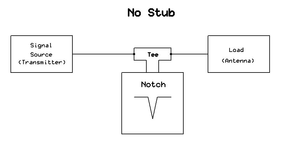
With a UHF "tee" connector right at the notch resonator (connected as depicted in Figure 5) one gets the results shown in Figure 4, below:

Figure 4:
The "notch" response with no stub between the Tee and the notch resonator.
Click on the image for a larger version.

As seen in Figure 4, the notch has relatively little effect in the upper end of the band (above about 14.2 MHz) - which is as it should be - but the notch depth is only around 6 dB in the CW/digital segment - again, a result of the resonator's limited "Q" and other factors that reduce it from the ideal.

Figure 5:
Notch with no "stub" - the result being shown in the plot
of Figure 4, above.
Click on the image for a larger version.

Fortunately, there's something that we can do about this:  Change the impedance at the resonator in our favor.

If one takes a look at the red circle, we can see that the resistance at marker #1 is in the area of 15 ohms.  If we apply a length of transmission line, we can use it to transform the impedance at the "Tee" connector to do a better job of shunting RF at a particular frequency.

Here's what happens if a 1/4 wavelength stub is connected between the "Tee" and the notch filter, connected in the manner depicted in Figure 7:

Figure 6:
The "notch" with a 1/4 wavelength stub inserted between the Tee and the resonator.  As we can see, the notch depth is greatly increased - around 25dB - but the response isn't particularly useful!
Click on the image for a larger version.

Adding the 1/4 wavelength stub of RG-8 type cable greatly increased the notch depth - around 25dB - and this is evidenced by the fact that the red marker (#4) shows, in the circle, an impedance of just a few ohms.  Unfortunately, this has two undesired effects:

Figure 7:
A stub between the tee and notch element.  As can be seen
in Figures 6 and 7, the length of this stub can change
the depth of the notch and the "shape" of the notch and
the attenuation of the nearby frequencies that are not
to be notched out.
Click on the image for a larger version.

• The frequency "distance" between the notch and the peak is now too wide - greater than the width of the 20 meter band.  This means that this configuration is not really usable for our intended purpose.
• There is now an asymmetry in the response:  The "peak" (minimum attenuation) is lower in frequency than the notch.

Also note that an upward frequency shift of the notch occurred due to various factors - mostly the reduced "loading" of the resonator - but because I was interested in the shape of the response rather than the actual frequency,  I did not retune the notch to the target frequency.

What about using something shorter than a 1/4 wave to do a less-dramatic transformation?

Figure 8:
The same arrangement as in Figure 4, but with a shorter cable - one that is approximately 0.15 wavelength.  The VSWR is acceptable with radios with built-in tuners - but careful adjustment of coupling and stub length could bring more of the red circle to the 50 ohm "center" of the green circles of the Smith plot.
Click on the image for a larger version.

In figure 8, a shorter cable was used - one that was about 0.15 wavelength of RG-8 type cable.  As figure 8 shows, the attenuation isn't as great - around 10 dB - but we we see that there is minimal effect on frequencies above 14.2 MHz and we see something else that is interesting:  An asymmetrical response that works in our favor:  There is less attenuation above the notch - where our SSB operation is to occur - than below it.  This "trick" is frequently used in notch filters - such as those used for repeater duplexers - to increase both the notch depth and provide an asymmetry that favors the frequency at which one wishes to have the least amount of attenuation, typically done with the use of parallel (shunt) capacitance and inductance - both being things that I have yet to try with these filters.

Its worth noting that even though there was a frequency shift with this stub, it was much less than that depicted in Figure 6, so I was able to easily re-tune it.

Two notch filters cascaded:

As it happens, I do have two devices that may be used as a notch resonator - the second one being the band-pass resonator - if I use only one of its ports.  The results are as follows:

Figure 9:
The result of cascading two notch filters.  The insertion loss is only slightly higher, but the notch depth is now over 20dB.
In reality, the second "notch" filter was just the band-pass filter with only one of the two ports connected.  A bit more tweaking would likely have reduced the insertion loss and brought the "pass" frequencies' matches closer to 50 ohms.
Click on the image for a larger version.

In this test I placed two notch filters in succession as depicted in Figure 10 - using 0.15 wavelength stubs between the two "tee" connectors (and notch resonators) and between the tees and the resonators themselves:  For some reason, I seem to have a bunch of RG-8 jumpers of about that length - around 0.15 wavelengths at 20 meters, which works out to be in the area of 7-8 feet (a bit over 2 meters) physical length, so that is what I used.

Figure 10:
Two notch elements connected with stubs to improve performance.
With properly selection of stub length, not only can the notch depth be "greater than the sum of the parts", but the actual shape of the response can be adjusted.  For Figure 9, all of the stubs had an electrical length of approximately 0.15 wavelength - but no additional testing was done with other lengths at this time.
Click on the image for a larger version.

As Figure 9 shows, the notch depth is a bit over 20 dB and there is only a slight increase in insertion loss to the 20 meter SSB frequencies:  Clearly, this configuration is definitely having a significant effect on the undesired CW/SSB signal and would probably solve most in-band overload issues!

Final comments:

No doubt different (better!) results could have been obtained with different stub lengths and configurations along with the use of parallel (shunt) capacitance and inductance to produce an asymmetrical  responce, but I have only so much time and not all that many random chunks of cable on hand and, more importantly, until(?) I construct another notch and pass resonator, I won't be able to use two cavities in the field.

One thing that is difficult to predict before-hand is the effect of source and load impedances other than ideal 50 ohm resistive that would be present with the output (transmit) and input (receive) impedances of HF transceivers, which are "nominally" 50 ohms:  In reality, these impedances can vary quite a bit (even between receive and transmit on the same radio!) and these differences can have an effect on the precise amount of attenuation that will be seen.  Practically speaking, it will be the transmit loss that will be considered - and this will also be affected by the radio's built-in antenna tuner, if it is inline.  Yet another factor that will affect the performance is the match of the connected antenna - particularly as seen at the far ("radio") end of the feedline - especially if a tuner is used there, too.

* * *

What would I do different if I construct more of these things?  As noted in the original June 30, 2014 blog entry (linked here) a major weak point of these resonators is the physical construction of the capacitive coupling probes:  They are not easy to adjust, and they are quite fragile - a good "jar" of the filter (pun intended!) can knock things out of position and cause detuning.  Having a means of being able to adjust the coupling without disassembly - perhaps the use of plastic screws accessible from outside the filter - would be very useful, allowing both critical coupling and tuning to be better-achieved while greatly improving ruggedness.

Perhaps, that will be a future project.

* * *

This page stolen from ka7oei.blogspot.com

[End]
 

Applying outboard AGC and filtering to RTL-SDR dongles to maximize usable dynamic range on HF

An AGC system for RTL-SDR "wideband" receivers operating in "Direct" (Q-branch) mode.

 A quick description of RTL-SDR dongles:

Figure 1:
An "RTL-SDR.com V3" USB-based receiver - one of the better,
"cheaper" options out there.
This unit has been programmed and marked with its own,
unique (to the system) serial number.
Click on the image for a larger version.

The so-called RTL-SDR dongles are ubiquitous and versatile because they can cover (more or less) from a few hundred kHz to over 1.3 GHz using various on-device signal paths - but all of these signal paths have in common one important limitation - The A/D converter is only 8 bits.

Despite these limitations, they are attractive because they are cheap - from $4 for the "bottom end" and cheapest devices (which are far noisier than they could be) to well over $50 for units with frequency converters and a few other bells and whistles - including band-pass filters.  The devices that we are using are just $20 and are the RTL-SDR dongles sold by "RTL-SDR Blog":  These units have thoughtfully-designed circuit boards that minimize extraneous, spurious responses and include a 1ppm TCXOs for decent frequency stability as well as providing separate signal branches for "direct" and "quadrature" signal paths for frequency ranges below 30 MHz and above around 60 MHz, respectively.

Ideally, the maximum range represented by an 8 bit A/D converter is around 48dB - and this is approximately what can be expected from these devices.  As with most things in the real world, the actual answer to the question of "what is the dynamic range" is more complicated.

In reality, noise produced by the device reduce the number of usable A/D bits and thus the dynamic range - but due to what amounts to oversampling and the contribution of the noise that is always present on HF - which can effectively "dither" the A/D converter, the apparent dynamic range can "seem" to be somewhat greater - perhaps well over 50dB, under some circumstances - but having 50-60 dB or so of usable dynamic range is not nearly enough for reasonable performance on the HF bands under a wide variety of signal conditions.

"But the Dongle already has an AGC!" One advantage of using a dongle with an upconverter - a device that would, say, converter 0-30 MHz to the range of  125-155 MHz - is that it then places these signals within the range where the R820T chip can operate - and this chip does have RF filtering and a sort of AGC - at least by way of being able to have its gain adjusted by software. Aside from the frequency drift issues related to this frequency up-conversion mentioned elsewhere, the problem with this is that the R820T chip really isn't that "strong" in terms of  its ability to handle widely disparate signal levels.  While the RTL2832 chip does have an AGC or sorts, the gain of both chips in the signal path must be carefully controlled to maximize performance.  Unfortunately, the precise nature of how these all work together isn't well documented and the general consensus seems to be that at HF, it doesn't work all that well. While the built-in AGC can work, we decided to avoid combining the somewhat marginal performance of the R820T signal path and the unknown nature of the AGC operation with the already-marginal 8 bits of A/D conversion in favor of an external AGC system operating within the well-defined limits of the dynamics of these devices when they are operated in "direct" mode.

The problem:

In this specific case we are using the "Q" branch of the RTL-SDR dongle for direct reception of HF signals:  For the purposes of this discussion and to avoid the complication of a discussion about aliasing, we'll limit the frequency range to 30 meters (10.15 MHz) and lower - a range that encompasses what are, in the current low end of the sunspot cycle, the two most popular HF bands:  40 and 80/75 meters.

In some circumstances - and with careful adjustment of RF levels - the limited dynamic range of the RTL-SDR dongles is "almost enough" - but because HF conditions widely change, the "optimal" amount of signal getting into the dongle goes all over the map:  During the daytime on 40 meters, noise can be very low and there are very few truly strong signals, but in the evenings or mornings there can be very strong signals from high-power shortwave broadcast stations.  These disparate situations cause some problems:

• If one adjusts the signal level going into the dongle to optimize being able to hear weak signals during the day (e.g. the background noise of the band driving the A/D converter to 10-15% full scale indication) it is likely that strong nighttime signals - both amateur and broadcast - will (more or less) saturate the A/D converter (e.g. put it into the range of "clipping"), degrading performance considerably.

• If one adjusts the signal level into the dongle to accommodate the very strong signals (which is only a "best guess" as such signals can vary by 10s of dB) then the input level to the dongle under "quiet" band conditions will be so low that sensitivity will suffer and spurious signals can appear everywhere as too few A/D converter bits are being "tickled" causing images and intermodulation distortion.

As mentioned before, the A/D converter's 8 bits do provide roughly 50dB of overall signal-handling range, but using one of these devices on HF soon makes it clear that one must constantly adjust the input level to assure that that 50dB "window of usefulness" is in the right place.  Using 60 meters as an example again, a "quiet" band in a good location may yield around -107dBm of noise in an SSB bandwidth, but a powerhouse shortwave broadcaster's signal can be into the -35dBm range - nearly 70dB higher than the noise (and there may be more than one of these strong signals!) which represents a range of at least 70dB.  What's worse, taking into account the need to provide 10-15% of A/D deflection just on the background noise on a quiet band for the dongles to work properly (to avoid serious issues with quantization-related distortion) roughly half of the 50dB or so available to us is already "used"!


Applying an AGC (Automatic Gain Control):

Figure 2:
Inside the 4-channel filter and AGC gain block module.
The individual band-pass filters may be seen at the far end of the lid-mounted
PCB ground plane while the actual detection and control circuitry
is on the prototype boards in the foreground near the bottom of the picture.
Click on the image for a larger version.

Any RF-based digital direct-sampling (or analog!) receive system - to maintain optimal performance - must have its input levels constrained, which is to say that one must take into account both the lowest and the highest signal levels.  In some cases it is simply enough to amplify/attenuate the input levels so that the expected signals will always fall in that range - and this may be practical on VHF/UHF or microwave, but it is certainly not the case at HF.

Even if we were to use a higher resolution A/D converter, we would still want to do this to keep all of the input signals within the "sweet spot":  Direct sampling HF transceivers such as the Icom IC-7300 and IC-7610 must apply both "strong" band-pass filtering and input gain control to maximize their overall performance.  In general, the more signal we throw into the A/D converter, the better - as long as we don't overdrive it and cause (excessive) "clipping".

Such is the case with these RTL-SDRs:  For best performance, one must have BOTH "strong" input filtering centered around the frequency range of interest (the narrower the better!) and keep the signal levels in the "sweet spot":  A properly-designed AGC can do this.

In short, the signal path and method is as follows:

• The signal comes from the antenna.
• Bandpass filtering for the band of frequencies is applied.  The narrower the bandwidth and "sharper" the filtering, the better.
•  Important:  One should never connect a receiver - particularly one with limited dynamic range - to an antenna without a band-pass filter that is designed to limitf the applied signals to the range of interest. (In other words:  Don't waste your time trying to make an RTL-SDR dongle work on HF without a suitable HF bandpass filter for the frequency range of interest - no matter which RTL-SDR dongle you use, filter out all but the frequency band in which you are interested.)
• On the output of the filter is an electronic attenuator.
• The signal level on the output of the filter (which is also being applied to the dongle) is measured.
• If the signal level exceeds a set threshold, the amount of attenuation is increased to cause it to remain at/near that threshold.

In short, the above system prevents the combination of all signals from getting to the dongle from consistently exceeding a pre-set level.  In this way, one can run a bit of "extra" gain to get the best weak-signal performance, but prevent the system from being hopelessly overloaded when very strong signals appear.

A practical implementation:

To maximize performance of the RTL-SDR dongles used for HF reception at the Northern Utah WebSDR, a "prototype" module consisting of four bandpass filters and four AGC gain blocks was constructed - see Figure 2.

Bandpass filters for 90-80 meters, 60-49 meters, 41-40 meters and 31-30 meters were constructed "Manhattan Style" on pieces of glass-epoxy circuit board material as individual filter modules which were then secured to the main ground plane - a larger piece of PC board material mounted in the lid of a Hammond 1590D aluminum enclosure.  Three dividers - also made of circuit board material - provide shielding between each of the band modules.

Constructed on small pieces of phenolic prototype board are the circuits that detect the RF and derive a control current for the electronic attenuators.  These devices are mounted elevated above the ground plane and attached to the shield walls which provides good RF grounding and a DC return path:  Two smaller "walls" are located at the far ends to provide the two boards at the ends with solid attachment points.

Comment:

You can check out the device depicted in this article yourself - simply go to the Northern Utah WebSDR and listen on the "60 Meter" and "30 Meter" bands on WebSDR #1 and WebSDR #2, respectively, or to the "90/80 Meter" and "41/40 Meter" bands on WebSDR #3.  All four of these bands use RTL-SDR dongles with the described AGC device.

Figure 3:
Schematic of the gain control block.  See notes below if a "standard" DBM is used.
Click on the image for a larger version.

Circuit description:

Figure 3 shows the gain control block schematically.

The input signal passes through the band-pass filter (shown as a block) with its output connected to a doubly-balanced modulator module, U3.  These devices are nearly identical to standard diode-ring doubly-balanced mixers, except that they are optimized for operation as an attenuator or baseband modulator:  The attenuation through them is inversely proportional to the logarithm of the current applied to the "CTL" (control) port.  In this case I used the Mini-Circuits LRAS-2-75 modules, originally designed for 75 ohm systems, but they work just fine at 50 ohms as well - being chosen because they are some of the lowest-cost components of this type offered by Mini-Circuits Labs.  The "official" specifications of the LRAS-2-75 gives specifications down to just 10 MHz, but it works fine at 3 MHz with just an extra dB or two of insertion loss.

Figure 3 gives a list of other suitable devices - some of which are rated down to lower frequencies than the LRAS-2-75.  Figure 3 also mentions the use of a standard doubly-balanced mixer such as the Mini-Circuits SRA-1:  A standard mixer will also work "acceptably" in this role if that is all that is available - but they tend to do worse at overall higher signal levels and one should attempt to find a proper attenuator like the LRAS-2-75 or similar.  If a standard doubly-balanced mixer is used, make sure that it has a port that provides a direct connect to its internal diodes to which the bias may be applied:  While this is usually the "IF" port, some devices have this particular port otherwise designated.  The presence of the diodes can be easily checked by using the "diode" function of a DVM between the device ground(s) and the control pin, observing a 0.2-0.3 volt drop in both directions/polarities of the meter.

The output of the attenuator (U3) goes two places:  To the RTL-SDR dongle being used for reception, and to the input of U2, an Analog Devices AD8307 logarithmic amplifier.  This device's input impedance is quite high, so a 470 ohm series resistor (R6) is used to lightly "tap" the RF coming out of the U3 while causing minimal circuit loading.  Included across the input pins of U2 is a low-value capacitor - typically in the 33-56pF range (as noted on the diagram) that is connected very close to the device to quash its response at VHF/UHF while minimally affecting HF signals:  Without this capacitor, U2 can easily detect any local FM or VHF/UHF TV broadcast signal - or even local VHF/UHF amateur transmissions - and be somewhat "desensed".  Practically speaking, this may not be a problem - particularly when it is placed inside a shielded container, behind bandpass filtering - but this can be distracting when the circuit is on the workbench being tested.

The output of U2 is a logarithmic response of the total RF energy (after having been passed through the filter) being applied to its input, the voltage increasing by approximately 250 millivolts for every 10dB of increase in signal:  If reasonable construction techniques are applied, signals well below -70dBm can be measured.  Because the maximum signal level (e.g. A/D converter clipping) of the "RTL-SDR Blog" dongle is in the range of -40dBm, no additional RF amplification is necessary in front of U2.

Figure 4:
Two of the gain control modules with U2, the AD8307s being
partially obscured by the ferrite beads.  These
beads are used to decouple any stray RF from the
common 12 volt supply line powering the modules.
Click on the image for a larger version.

U1 must be an op amp capable of operating down to the negative rail in order for this circuit to function and the specified LMC660 is ideally suited.  The DC output of U2 is applied to U1a, one half of a dual op amplifier, wired as a unity-gain follower to set a low impedance point, and this DC signal is then applied, via R5, a 1 Megohm resistor to U1b, which is configured as an integrator by virtue of a 0.1uF capacitor placed in the feedback path with the threshold being set by R4, a 10 turn potentiometer.  If the integrated DC signal from U2 is above the threshold set by R4, the voltage output of U1b decreases, reducing the bias applied to attenuator U3 and increasing its loss, but if the signal is below the threshold, the voltage increases, decreasing the attenuation.  By this action, the combination of U1 and U2's action will prevent the average signal at the bandpass filter's output from exceeding the threshold level set by R4.

Whereas a typical AGC found in a receiver will have a fast "attack" and a slow "decay", we want this AGC to be comparatively slow to respond so that it will (hopefully) not be completely deafened by the occasional static crash.  In reality, allowing the A/D converter to hit full-scale on occasional peaks will have minimal apparent impact on reception.  In the absence of broadband static crashes, the cumulative power within the bandpass filter's range will change comparatively slowly over time and it is this that we wish to track.

In the DC path between the output of U1a and the "CTL" pin of U3 is a series LED which provides both a bit of logarithmic current response intrinsic to semiconductor diodes as well as providing a handy visual indication of the state of the circuit:  If the LED is lit, attenuation is low, but if it is very dim or turned off, more attenuation is being applied.  In testing, the photosensitivity of LEDs was simply a "non issue" and ambient light had no discernible effect on circuit operation - and even if it was at all noticeable, it will be placed in a metal box, anyway.

Resistor R3 provides current limiting to the diode while R2 provides a current sink:  The combination of R1 and C1 (located very close to U3) terminate the "CT" port (at high frequencies) at the nominal impedance of the RF portion - in this case, around 50 ohms.  Also included is U4, a 5 volt regulator:  This supplies power for U2 as well as provides a stable reference voltage for R4, the RF threshold adjustment:  It need not be exquisitely stable with temperature as several dB change of the AGC threshold with varying temperature is of no importance in this application.

Under normal "quiet" conditions the RF level going into U2 will be too low to exceed the threshold, causing the output of U1b to go to maximum voltage, biasing U3 to set minimum attenuation - it is only in the presence of stronger signal(s) that the gain reduction will occur.

Circuit calibration:


To calibrate the circuit, a signal generator is required, the procedure being as follows:

• Pre-set the wiper of R4 (the 10 turn pot) to ground (zero volts at U1b, pin 5)

• Set a signal generator it to a frequency within the passband of the filter and an RF level of around -20dBm.

• Connect the input of the dongle to the signal generator and tune it to the frequency of the generator using software of your choice.  Make sure that the "direct - Q" signal path is selected since we are not using an upconverter.
• If using SDR-Sharp, tuning in the signal (using AM is best) "hovering" the mouse over it on the waterfall display should give a dBFS reading.
• If using the "HDSDR" program, the "dBFS" reading will appear on-screen in the receiver control panel.

• Using the software, monitor the level of the applied RF signal's "dBFS" (dB with respect to full-scale).  Ideally, a full-scale A/D indication would yield a dBFS reading of around -6dBFS, but it seems that the internal scaling of the signals from an RTL-SDR dongle aren't scaled, so the reading may be in the -30 to -50 dBFS range.  Monitor the "dBFS" from the dongle while increasing/decreasing the signal and note the highest value.  The goal here is to determine the reading given by the program.
• Ideally, one would like to be able to see the "recent-highest" reading of the A/D converter of the dongle, but this may not be available in the programs used with the dongle.
• If adventurous, one can use the "librtlsdr" tool called "rtl_sdr" and dump the results to a file or a display program to monitor the raw A/D values.
• If you operate a WebSDR using the PA3FWM software there is a utility that will directly read out the number that we want to look at:  Contact me directly for details.

• Having determined the maximum-displayed "dBFS" level, connect the signal generator to the input of the bandpass filter and the RTL-SDR dongle to the output (e.g. J2 in Figure 3) with the frequency set to the center of the desired frequency range (usually - but not always - the middle of the filter's passband).  The amplitude of the signal generator is set for level higher than one would reasonably expect to see on the input - say -20dBm.
  

• At this point the LED should not be illuminated and U3 will offer maximum attenuation.

• Slowly increase R4 until the LED just starts to be illuminated.  Watching the "dBFS" reading, adjust R4 for a signal level that is about 6dB below the maximum reading that you'd previously obtained.  Ultimately, you will want to set the peak A/D output to between 1/4 and 1/2 of full scale which represents -12 to -6 dBFS, respectively.

• If the circuit is working properly, any signal above that corresponding with the threshold should be limited at the set value by automatically setting U3's attenuation, but a total signal power level below the threshold should cause U3 to operate at minimum attenuation as indicated by maximum LED brightness.
• If you are using a signal generator with a built-in "step" attenuator, changing signal levels may cause momentary "glitches" of high signal that may cause a momentary disruption in the A/D reading and slightly upset the AGC:  Simply wait for a few seconds after making an adjustment for the readings to settle after making a change.

Figure 5:
Two bandpass + attenuator (U3) modules.
The inductors/capacitors of the filter may be seen in the
middle of the individual boards while the attenuator (U3) is the
white object seen in the lower-right corner of each board.  U3 is wired
"dead bug" style in each case.
Click on the image for a larger version.

Observations in use:

So far, these devices seem to be working as intended.  Even with higher overall gain in the signal path than before (e.g. when band conditions are poor and/or there are no strong signals in the filter's passband) the RTL-SDR dongles have not been observed to show obvious signs of overload when extremely strong signals are present - this having been a problem previously.  Initially, the AGC threshold was set for -6dBFS (1/2 A/D scale) using a CW signal from a test generator.  In the weeks that followed, these receivers were monitored during high-signal conditions and it was noted that there had been no obvious problems.  The AGC threshold was later reset for -12dBFS (1/4 A/D scale) and an additional 6dB of RF applied to the receivers with no obvious degradation in performance in the presence of strong signals, but a slight improvement in weak-signal performance when the bands were "closed".

In looking at receiver stats, there are still instances of A/D "clipping" - but this is to be expected:  The AGC circuit integrates the level over time (perhaps a few seconds) and brief excursions well above the threshold level are to be expected, both from static crashes, but also coincident modulation peaks of several strong shortwave broadcast signals.  Because the "occasional" clipping typically has little apparent impact on the receive signals (particularly the narrowband signals on shortwave frequencies) this effect isn't usually noticed.

On some of the bands, a bit more RF signal is needed to optimize performance - that is, to "tickle" more A/D bits when signals are weak.  Previously, doing so would risk gross overload of that receiver when the band "opened" with strong signals, but the AGC block should minimize any such issues.

Not mentioned previously, this AGC system can skew the S-meter readings from the receiver somewhat.  In the presence of strong signals, the AGC will lower the overall system gain causing the readings to vary and appear low.  In theory, one could monitor the voltage being applied to bias the attenuator and relate this to the amount of attenuation and offset the S-meter readings, but this may be overkill in most situations!

---

The above article was posted (by me) as a technical article at the Northern Utah WebSDR (link).

While the circuitry could be integrated onto a small circuit board, this has not been done as the circuits are quite simple and easy to construct as depicted.

* * *

This page stolen from ka7oei.blogspot.com

[End]

Quieting an insanely (RFI) noisy LED floodlight

A friend of mine recently installed some inexpensive Chinese-made floodlights to illuminate his backyard, but was dismayed to discover that when they were on, his 80, 40 and 20 (shortwave - 3.5-14.5 MHz) reception "went away", replaced with a very strong noise that was "20 over" - a degradation of apparent sensitivity of much more than 20dB.  As it turned out, almost every frequency below and above this range he checked was also affected to a similar degree.

RF noise from "grow lights" - the same phenomenon Several years ago, there was some noise (pun intended) in the Amateur press about LED power supplies being sold that caused a tremendous amount of RF interference - and many of these stories also included anecdotes of many of these interference sources having been tracked down and found to have been "grow" operations.  Later, some stories surfaced where law enforcement officers were able to locate some of these "grow ops" simply by finding the source of RF interference. The LED power supply described on this page is of the same type that was found to cause these very high levels of RF interference.

Even though these lights aren't turned on very often, he decided that their flaws went firmly against his eternal crusade against RFI-generating devices at his house.  After all, when it comes to RF interference, one should remember this cardinal rule:

Most RFI begins at home!

To be sure, there are many cases in which there are noisy power lines or a neighbors plasma TV - just two in a long list of things that can cause interference, but the worst offenders in generating interference are likely in one's own house.   The main reasons for this are simple and (for the most part) obvious:

• They are nearby.  If a noise generating device is in your house, it's very close-by - and the closer it is, the more your antenna is likely to intercept "grunge" from that device.

• They are connected to the same wiring as everything else in your house.  There's nothing like a piece of copper to convey RF all over the place with minimal loss, and if a noise generator is powered from the mains, it's likely conducting much of that noise into the same mains connections that power your radios.

• If you are like most amateurs, you probably have radiating feedlines on your HF antennas.  By their very nature, almost all HF antennas tend to radiate a bit of RF on their feedlines.  For some antennas (e.g. dipoles, yagis, loops) this is incidental - often due to inadequate balun design, but other antennas (offset-fed antennas like Windoms, end-fed antennas) this is often by nature or design.  If the feedline of your HF antenna isn't very well-balanced (often using a "current mode" choke) some of your "noise" from the devices in your house wiring is being conducted from your shack, onto the feedline and then into your antenna.  Fixing this problem certainly warrants a series of articles itself, but suffice it to say, "noisy" devices will seem worse because of this issue than they would normally be.

Figure 1:
The constant-current LED driver with added filtering.  This LED driver
is typical of what is seen in these devices:  A rather generic, potted module
of likely-questionable lineage and quality.
Click on the image for a larger version.

What are these things?


As is typical with these inexpensive LED lamps, the power supply is a constant current module that uses PWM/switching techniques to regulate the current applied to the LED array to some value.  As can be seen Figure 1, this is simply a box with two sets of wires:  The AC (main) input on one side and the DC output to the LEDs on the other.

Because these are constant current supplies, they can be used over a wide range of LED module voltages:  22 to 36 volts, according to its label of that in Figure 1.  Noting the official "50 watt" power rating, we can do the math and see that with a constant 1500mA, the power being delivered to the LED array can vary from 33 to 54 watts, depending on its actual operating voltage.  Depending on the design, these supplies may or may not have their DC outputs isolated from the mains input via an internal transformer, so it is best to assume that they are not isolated and that the DC outputs will be line-referenced and hazardous (even lethal!) to touch.

In this example, the red and black DC leads disappeared into the body of the case where it would connect to an LED module that is (presumably!) insulated from the lamp's case.  Because you can't be sure what to expect, one must always make sure that the safety ground of these lamp housings is actually connected to the case (the ground wires in these devices are often not connected to the case at the factory!) and that it is plugged into a GFCI-protected outlet.

How bad was it?

In the case of these LED floodlights, the only connection that they had to the rest of the universe was via their power connections, so it was clearly via its power leads that they were radiating their "grunge".  To determine in some quantitative way how noisy this device was, a simple test fixture was constructed to measure the energy imparted on the mains power lead, represented schematically in Figure 2, below:

Figure 2:
Test fixture to analyze the amount of RF being conducted from the LED's current supply to its mains leads..
"Ca" and "Cb" are 0.1 to 0.47 "X" class "safety" capacitors used for mains filtering and "La" is a bifilar mains choke of at least 1 milliHenry per winding, these constituting a filter to decouple noise already present on the mains from the test fixture:  One of the filters depicted in Figure 5 could have been used for this purpose.
RF coupling transformer "Ta" consists of a Mix 31 clamp-on ferrite choke with a single wire going to the "Device Under Test" as the primary and 6-8 turns of smaller wire as the secondary to couple RF from it.  The box marked "protection" is simply two back-to-back 5.1 volt Zener diodes in series to protect the analyzer from voltage transients caused by turn on/off transients.
Click on the image for a larger version.

In this circuit we see a common-mode line filter using Ca, Cb and La forming a circuit to attenuate noise that might already be on the mains.  The goal is that when we measure RF noise via coupling transformer Ta, we are (mostly) seeing the noise from the device being tested and not that which may already happen to be on the mains.

The result of this measurement can be seen in Figure 3, below, covering the range from nearly DC to 1 GHz, with the cyan trace being with the unit turned off and the yellow trace with it turned on:

Figure 3:
Noise from the power supply as seen from 0 to 1 GHz.  The blue trace is with the LED power supply powered down while the yellow trance shows it powered up.  As can be seen, it is a potent noise generator well into the UHF spectrum - but particularly at and below 100 MHz!
The various signals on the cyan trace are off-air signals, including AM, FM and TV broadcast and 800 MHz - plus some leakage from the noisy mains through the Figure 2 filter:  Ingress of these signals is the inevitable consequence of the rather simple lash-up and not conducting these tests inside an RF-screened room!
Click on the image for a larger version.

While this test fixture isn't perfect (e.g. some leakage from the mains through the filter, some couple of broadcast signals directly into the fixture over the air and the fact that the coupling coefficient is unknown because I didn't bother to determine it!) it did the job of giving a relative indication of how much "grunge" the LED's power supply put into the mains - and this same information would later be useful to get a general idea as to how much our mitigation efforts reduced this noise.  As can be seen, below 100 MHz the added noise (in a 3 MHz detection bandwidth) is nearly 50dB (100000 x) higher than the noise floor of the analyzer and the test fixture.

Refocusing on a smaller frequency range with different analyzer settings, let's take another look at how bad it is over the lower HF range:

Figure 4:
A re-done plot over the range of 0-100 MHz, this time with an 8 MHz resolution bandwidth.  The higher resolution bandwidth results in a higher reading from the QRM generator as its output is broadband noise.
Over much of this range, the base noise level (in cyan) is below the measurement sensitivity of the analyzer.
Click on the image for a larger version.

From the plot in Figure 4 we can start to get a picture of how bad the situation really is.  As can be seen at Marker #1, we measured a power level of about -3dBm - or 0.5 milliwatts within an 8 MHz bandwidth, but if we were to integrate this energy over the entire 0-100 MHz range we can see that there may be, perhaps a couple of 10s of milliwatts of noise being coupled into the mains:  We can only guess at the true amount of conducted RF owing to the comparative crudity of our test fixture and its unknown coupling coefficient across the RF spectrum, but we can be reasonably sure that what we see on this trace is but a fraction of the total energy present.

Figure 5:
Some board-mountable Shaffner mains filters from the Electronic
Goldmine, item G21844 (no longer available - sorry...)
Click on the image for a larger version.

As noted earlier, the entire purpose of these measurements was not to determine an absolute level of RF energy, but rather to have a means of repeatably measuring how bad things are - and also to be able to determine if our mitigation methods are having the desired effect.

"Fixing" the problem:

One solution to this problem (aside from not getting cheap, uncertified devices in the first place - but even then, one is never sure what one is really buying!) is to add known-to-be-effective filtering to the mains leads.

At about the time my friend brought these lamps to me, I noticed that the Electronic Goldmine had, on sale, some small, board-mount mains filters, so I suggested that he buy at least two for each of his three lights (for a total of six) - so he bought 10 of them.  These particular devices were attractive because they were relatively inexpensive, potted (helpful, because this will be mounted outdoors where moisture ingress could be a problem) and small enough to fit in the limited-space enclosure in the back of the floodlight.  Being that the lamps were only "50 watt", the 1.6 amp rating of these filters would be more than adequate.

Figure 6:
Another view of added filtering and their integration into the enclosure.
The Shaffner filters were mounted "dead bug" (leads up) and held in place
using both the ground wires and silicone (RTV) sealing compound.  The
lug at the lower-right was added to help make sure that this plate was
electrically bonded to the main body of the LED floodlight.
Click on the image for a larger version.

As can be seen in Figure 1 and Figure 6, two of these filters were installed "back to back" in the back of the lamp housing, using direct-soldered connections between the ground terminals of the filters and the metal plate itself with short pieces of heavy (8 AWG) copper wire to keep the impedance of these leads as low as possible:  Even a few inches/centimeters extra was found to significantly reduce the efficacy of these filters at VHF and higher frequencies.

You may notice something else about the layout:  The wires going in and out of the LED driver are bundled together with plastic wire ties and routed to the "far" side of the power supply, as distant from the mains filters and wires as possible - this to minimize the amount of RF energy that might be coupled from these "noisy" wires into the power cord - something that would surely "un-do" some of our hard-won efforts in minimize the amount of conducted RF noise.

The result:

The results of this effort can be seen in Figure 7, below:

Figure 7:
"Before" and "After" traces over the 0-10 MHz range.  The cyan trance is with the LED unit powered down, the yellow trance is without filtering and the magenta trace is including filtering.  Note the lower resolution bandwidth (91kHz) as compared to the other figures which will tend to reduce the apparent level of broadband noise from LED driver and accentuate those of "coherent" signals such as broadcast stations.
The strong signals at about 1.0-1.4 MHz are due to ingress of local AM broadcast stations into the lashed-up test figure, the level exceeding that of the leakage through the filter.
Click on the image for a larger version.

In Figure 7, above, we can see multiple traces - with the explanation below:

• The Cyan (blue-ish) trace is our baseline measurement with the LED driver module powered down.  The signals below about 1.5 MHz are ingress from strong, nearby AM broadcast stations, some of which are nearly as strong as the noise at specific frequencies.
• The Yellow trace is with no filtering of the LED driver module, showing the relative energy from the LED driver module over the 0-10 MHz range.
• The Magenta (purple-ish) trace is with the LED driver module powered up with the added filtering.

"Could you have just snapped ferrites on the power cable?" In reading this article, one might wonder if we could have solved the problem simply by putting snap-on ferrites on the power cord. I doubt it. Snap-on ferrite devices are very good about reducing the amount of RF conducted on wire, but with the extreme nature of the interference of these devices, it would never have been enough at HF.  The reason for this is that in order to adequately quash the QRM to the "point of undetectability" it would take at least several k-ohms of impedance on the power cable to solve the problem. While it is possible that one can do this, it would take several large-ish cores (probably mix 31) with a dozen or more turns on each just to add that much reactance - but that material and winding topology would only work to the high end of the HF spectrum, so you'd need another core or two with windings on different materials - say 43 and 61 mix. To make matters worse, you'd have to keep these chokes well-separated physically or else RF energy would be conducted around them - or even radiate directly from this rather large structure:  You certainly wouldn't have been able to easily fit it in the back side of the lamp's enclosure. Self-contained filter modules like the ones used are specifically designed to quash RF over a very wide frequency range:  Not only are bifilar inductors used, but capacitors are also used to force the interfering energy to common mode so that the inductors can best do their job, plus there are other capacitors that do an excellent job of shunting RF to the case to "completely" contain that energy. In other words:  In such an extreme case, you'd be far better off using an L/C filter like that depicted in Figure 5 without even bothering with ferrite chokes.

Interpreting these results we can see that over much of this range that the filtering reduced the amount of conducted noise to just above that of the cyan line, knocking the noise down by roughly 20dB over the range.  These filters start to lose their effectiveness below 1 MHz which is why, at very low frequencies (below 500 kHz) one starts to see more conducted energy - but these frequencies don't radiate very well, anyway so they are of generally less concern in most amateur stations.

When this plot was taken, the circuit depicted in Figure 2 was very close to the filter networks and it was believed that some energy was directly coupling into it from the LED driver module.   After the lamp was assembled (the cover put on and the power cord fitted) another test was done and no difference at all could be seen in the "on" and "off" traces - except at frequencies below about 1.5 MHz:  I somehow managed to omit capturing this trace.

Did it help?

Yes!

My friend reinstalled these lights and was happy to report that upon listening on various HF bands from 160 through 10 meters, he was unable to detect when the lights were on or off, indicating that the modification was successful.  It is possible that within a few feet/meters of these lights that some low-level direct radiation of noise could have occurred on VHF/UHF frequencies, but this energy was demonstrably not being conducted via the power cord, and emissions would not likely be detectable more than a few feet/meters away, anyway.

Would just a single  filter have done the job?

Probably - but since the lights were a bit of a pain to take down and put up again it was decided to use two of these filters just to avoid the possible hassle of having to take them down (and apart) again if just one filter hadn't been enough! 

Follow-up:

It would seem that the statement above about questionable quality was justified:  In the two years since these were installed, only one of these lights continues to work, the other having failed in fairly quick succession.

The phrase "Caveat Emptor" comes to mind!

* * * * * * * * * * *

Links to other articles about power supply noise reduction found at ka7oei.blogspot.com:

• Containing RF noise from a "pure" sine wave UPS.   Even when it is not operating your sine wave UPS may be producing a lot of HF radio interference!
• Completely containing switching power supply RFI - link.  Sometimes it can be difficult to quiet a switching power supply, so it may be necessary to put it in a box with strong filtering on all of the conductors that enter/leave.
• Minimizing VHF (and HF) RFI from electronic ballasts and fluorescent tubes - link.  Electronic light ballasts, like many switching power supplies, operate in the LF frequency range so "cleaning them up" at VLF/LF/MF frequencies can be a challenge.
• Quieting high current switching power supplies used in the shack - link.  This page describes techniques that can be used to reduce the amount of RF energy produced by switching power supplies that you may be using to power your radios.  Again, higher-inductance chokes may be required at VLF/LF/MF frequencies.
• Reducing switching supply racket - link.  This describes techniques that can be used to beef up the filtering for switching supplies in general.
• Quieting a 150 watt Samlex sine wave inverter - link.  This page talks about making an RF-noisy sine wave inverter RF-quiet.
  

This page stolen from ka7oei.blogspot.com

[End]

A 2 meter and 222 MHz low-pass filter for the SocoTran ST-7900D

In an earlier post (link) I described a "hilariously bad" radio - the Socotran ST-7900D (a.k.a. the QYT "KT-7900D").  This radio, right out of the box, could not legally be used by U.S. amateurs on three of its four "bands".


One of these bands - that which covered 350-390 MHz - was understandably off-limits as there is no U.S. amateur band in this frequency range but the other two, the 2 Meter and the 1-1/4 meter (a.k.a. 222 MHz band), also covered by this radio, had poorly-filtered harmonic content:  It was even possible to key up a fairly-distant UHF repeater when one transmitted on a 2 meter frequency at precisely one-third of its input frequency!

The article noted that as it was shipped, the only band that might be legally used was the 70cm band as the strongest harmonics of the other bands weren't properly suppressed - not at all, actually...  It was observed that this radio seemed to have a single low-pass filter in its transmit path that was designed to start cutting off energy in the 550-575 MHz range - but this sort of filter would have no effect at all on the 2nd and 3rd harmonics on 2 meters and the 2nd harmonic on 222 MHz - which was the problem.

Besides just being cheap, one reason why someone might have been attracted to this radio is its ability to operate in the 222 MHz band - and paying $75 or so for a  25 watt radio that could only do 222 MHz might be a reasonable thing to do - so what about making some sort of low-pass filter that would kill two birds with one stone:  A single filter that would allow legal operation on both 2 meters and 222 MHz without having to switch filters?

Designing the filter:

What I needed was a filter that would pass the 222-225 MHz band with little attenuation, but still knock out the 2 meter band's 2nd harmonics in the 288-296 MHz range.  This sort of filter would permit operation on both the 2 meter and 222 MHz band without needing to switch or change anything - but if would, of course, preclude operation on 70cm unless it were removed.

Curious to see if this could be done I fired up the Elsie program, a software tool that is free for "student", non-commercial use (aren't we all students in this world?).  Designing a filter that would both adequately attenuate 2 meter's 2nd harmonics and pass 222-225 MHz would require at least a slight amount of complexity, so I went to work.

Knowing that a simple Butterworth or Chebychev filter would never meet the need for "sharpness", I immediately picked a Cauer (a.k.a. "Elliptical") low-pass filter design and plugged in the numbers, coming up with this:

Figure 1:
 Low-pass filter, inductor-input topology shown.  This "same" filter could have been constructed using capacitors on the input/output, but this version uses fewer capacitors and more inductors - which are both extremely cheap to make and are very easily adjusted - unlike fixed capacitors.
Click on the image for a larger version.

When I plotted the predicted response of this filter, Elsie showed me this:

Figure 2:
The predicted attenuation of the filter.  Part of the design goal was to place the 2 meters' second harmonics in the first "notch" in the filter.  While only 40dB was theoretically needed, a filter with 50dB attenuation was implemented knowing full-well that the real-world implementation of the filter may not do quite as well.
Click on the image for a larger version.

While I needed "only" 40dB to make this radio "clean enough" it is often the case that real-world filters aren't quite as good as their simulated counterparts, so I inputted 50dB into the program as the minimum attenuation.  If you look closely, you'll see that at the top of the flat part - just before it "rolls off" - the attenuation at 232 MHz, comfortably above the 222 MHz band, is just under 1dB while there is a deep "notch" at around 290 MHz - which is right where the 2nd harmonics of the 2 meter band will lie.  If this filter was, in fact, "build-able", it would neatly solve the problem of the harmonics from the 2 meter and 222 MHz bands.

When it came to specific filter types I had two choices for the "same" filter:  A capacitor-input low-pass filter and an inductor-input low-pass filter.  Both are theoretically equal in performance, but because the capacitor input version had 7 capacitors and the inductor input version had just 3 capacitors, I chose the latter as seen in Figure 1:  Inductors - which are just a few turns of wire - cost practically nothing to make and are easily adjusted!

Being familiar with VHF/UHF construction techniques I knew, when I saw the inductor values, that they would be very small, but easy to make.  For example, when 20 AWG wire is wound on a 3/16" (4.76mm) diameter drill bit with very short leads, you can expect to start with something along the lines of:

• 20-30nH:  2 turns
• 30-40nH:  3 turns
• 40-50nH:  4 turns

The precise value would then be obtained by squeezing/stretching the turns - or, possibly cutting a fraction of a turn off as necessary.  If you have ever looked at some commercially-made VHF/UHF gear you might have noticed that some of the coils look as though they were smashed or stretched, but this is a time-honored way of making fine adjustments to these circuits after assembly.

If one is constructing this using only small, surface-mount components the self inductance and stray capacitance of these tiny components on a well-designed board can almost be ignored at these frequencies - but I was going to use plain, old through-hole leaded disk ceramic capacitors, which would require a bit more consideration.

A good example of this is the first series-resonant section of the above filter - in the section marked "531.581M".  As you can guess, this is a series-tuned circuit that must be resonated at around 532 MHz using components of the approximate values shown.  Practically speaking, in this application one can "fudge" a bit on the values, so rather than trying to find a precision capacitor of about 17.5pF, I simply pulled a 18pF unit out of my capacitor bin with the idea that I would select the inductance to make it resonate somewhere in the area of 532 MHz.

But, there's a twist:  Noticing that resonating inductance is ideally 5.1nH, one may realize that even a rather short length of wire has a similar amount of inductance - and that is exactly what was done:   The capacitor's own lead - about 4 millimeters of it - plus the series inductance of the capacitor itself was enough to create a resonant circuit at the desired frequency.

What it takes to build this filter:

As you may have gathered, it is simply not possible to build this filter without some sort of test equipment at hand - and I used a spectrum analyzer with a tracking generator as I was building it.  In short, here's what I had to do:

• Fuss with the series L/C circuits to get the stated series resonant frequencies as indicated by deep notches on the sweep.
• Stretch/compress/adjust the other inductors as necessary to minimize the loss below the cut-off frequency
• Repeat the above two steps until it makes no difference - usually taking about a half-dozen iterations.

During construction I didn't bother breaking out any capacitance or inductance measuring gear - but very small inductors (those lower than a few hundred nanoHenries) can be very difficult to measure, anyway.  Using only "known" values of capacitance, by adjusting the inductors in the manner mentioned above, I have found via experience that such filters often "take care of themselves" when one takes a bit of care during assembly and adjustment - particularly when setting the resonant frequencies of the "notch" elements.

Amazingly, the filter went together without too much trouble with the test equipment indicating less than 1dB of insertion loss at either 2 meters or 222 MHz.  The hastily-kludged prototype looks like this:

Figure 3:
Constructed prototype.  This was constructed on a scrap piece of copper-clad PC board material using small PC board islands for some component support.  This version was built for testing the concept:  A "real" implementation of this filter would be crammed into a small metal box with the input/output inductors and ground plane soldered directly to the in/out RF connectors.
A circuit board could be designed, but to be effective it would need to be built on (at least) a double-sided board with a large-as-possible ground plane on the top connected to the bottom plane using lots of vias.
Click on the image for a larger version.

Figure 3 shows the prototype, constructed on a small piece of copper-clad circuit board material.  The input/output connections were made via some N connectors that were pre-attached to UT-141 rigid PTFE coaxial cable, being were used because they were on-hand.  Because we would need to handle "only" 25 watts, 100 volt NP0/C0G disk ceramic capacitors are more than adequate.

As can be seen in Figure 3 the junctions where the series L/C portions are attached are held off the ground plane with small pieces of circuit board (the capacitive effects of these are negligible at these frequencies) while the attaching hardline's center conductors supported the in/out inductors.  Also apparent is what looks like haphazard stretching/compressing of the various inductors to achieve the resonant frequencies for the three elements - which I marked on the board.

Once I connected it to a transmitter I did a bit of final tweaking, "adjusting" the series coils for minimum loss (as indicated on an RF power meter) on both 2 meters and 222 MHz but leaving the "notch" adjustments alone:  Only slight adjustments were needed.

Can I make such a filter?

Yes, you can - if you are familiar with VHF/UHF circuit techniques and have access to a spectrum analyzer with a tracking generator or some sort of equivalent.

If you don't have access to this sort of gear - and you don't know anyone else who does - then it is (unfortunately) not possible to properly "tweak" this filter for both harmonic attenuation and also to make its insertion loss and added VSWR low enough to both allow transmit power to pass through it without damaging the radio.

(And no, I won't build one for you...  Remember:  It's a $75 radio!)

Does it work?

Amazingly enough, it works pretty much as predicted!

After final tweaking the measured insertion loss was under half a dB:  With 25 watts in, around 20 watts exited the filter on both 2 meters and 222 MHz - hardly enough loss to worry about on receive or transmit.  After about a minute of solid key-down at 25 watts input the hottest of the filter's components were barely warm - lower than body temperature in a "not hot/not cold" room.

The real test was to put the filter inline and check it again on the spectrum analyzer - and the plots below show the results for 2 meters:

Figure 4:
The harmonics on 2 meters, through the filter.  The analyzer has been adjusted to read actual power, so the 2 meter fundamental is at about +43dBm.  The second marker (#2) shows the location and amplitude of where the 2nd harmonic would be - and this trace shows that it is at least 79dB down well within the FCC part 97 rules and  probably "cleaner" than your average "good" radio!
Click on the image for a larger version.

And here is the result from the 222 MHz band:

Figure 5:
The operation of the radio on the 222 MHz band.  The "2" marker shows the second harmonic - and other spurious signals may be seen at a similar level on the plot.  Like the plot in Figure 4, this is scaled to show the actual transmitter power (+43dBm) and thus the harmonics and spurious signals are around 80dB below the carrier - well within FCC part 97 rules!
Click on the image for a larger version.

As can be seen, the harmonics and other spurious signals are all but undetectable!

"Sweeping" the filter:

Curious as to how the actual attenuation curve of the filter looks?  Figure 6, below, shows its response over the frequency range of 100 through 400 MHz.

Figure 6:
A "sweep" of the prototype filter from 100 through 400 MHz.  On this plot marker #1 has been configured so that the difference in amplitude being measured and this indicates that the depth of attenuation is a bit over 53dB - but the settings of the analyzer used to make this plot likely reduce the apparent depth.  Outside that null the depth of attenuation is at least 40dB - more than enough to suppress the harmonics to meet FCC part 97 regulations.  If I'd taken a bit more care in building the filter (e.g. more thoughtful layout, some shielding between sections) more attenuation might have been obtained - but as it was, it worked better than was necessary.  Because of the configuration of the test jig, the absolute level of the passband portion of the response is arbitrary.
Click on the image for a larger version.

As can be seen, the "depth" of the low-pass filter is at least 40dB, but where the first "null" is located (which happens to be around the frequencies of 2 meter 2nd harmonics) the depth is much greater.

As expected, the simulated filter's ">=50dB" attenuation above the designed cut-off frequency wasn't quite met over its intended range (likely due to the physical layout of the filter - not to mention the difference between simulated and real-world components) but it is more than capable of rendering this radio "legal" when it is operating on the 2 meter and 222 MHz bands.

Using the filter:

Some time in the near future it is likely that this page will show a version of this filter that is built into a small box with UHF connectors which will allow the radio to be used legally on 2 meters and 222 MHz by U.S. amateurs - but having this filter inline precludes its use on 70cm:  To do that, the filter would have to be manually removed.

If that is the case, one would consider this to be a "2 band" radio - and for around $75, it would to OK - aside from the possible tendency for its receiver to overload from nearby signals.

What about automatically switching the filter?

In theory, it should be possible to build into the filter a "bypass" circuit using some UHF-rated relays.

In poking about inside the radio I quickly found a circuit that was powered on only when the UHF (400 MHz) band was selected - and this could be used to "key" a relay to bypass such a filter.  In reality, one would want to design such switching so that when the relay was un-powered, the filter would be bypassed, but when the radio was powered up and not on UHF, use the absence of the aformentioned signal to pull in the relays in insert the filtering.

If we decide to do this, I'll post it here - but at some point, trying to make this radio do what it should have been capable of doing by design becomes an exercise of "turd polishing" when the time and money spent exceeds the gain.

Then again, the effort is sometimes worth the journey if the goal is to build and learn something!

(No, this filter won't help with the problem of this receiver being easily-overloaded by other signals in the same "band".)

* * * * * * * * * * * *

This page stolen from ka7oei.blogspot.com

[End]