What the heck happened to this Sense power monitoring module?

Figure 1:
The exterior of this Sense SM3 power sensing module.
The connections are made via barely-visible holes on the left side while a
WiFi antenna permits connectivity onto the user's wireless network.
Click on the image for a larger version.

A friend of mine had a "Sense" ^tm power monitoring system at his house for a couple of years.  This device works with additional software to allow a user to monitor power consumption within their house or business, potentially offering the ability to audit loads and manage their household power consumption.  It also has the ability to monitor the production of a rooftop solar, allowing another means of monitoring its production and performance.

This system and its software wasn't without its minor quirks - particularly with its attempts to automatically identify loads , but it did work pretty well.

Until recently.

A couple of months ago (around February, 2020) he started getting anomalous readings from the unit - and a day or two later, it failed to provide any current readings at all but it still read the mains voltage.  Upon opening his breaker panel he could detect the strong smell of burnt glass-epoxy circuit board so he knew that the unit had catastrophically failed in some way.

Figure 2:
The other end of the Sense unit showing the model number.
While masked for this picture, it appeared to be a
rather early production unit with a very low
serial number.  It would be interesting to know if that
fact was significant to this event.
Click on the image for a larger version.

He sent it in to the manufacturer to check about a repair and after a pandemic-induced delay of a monitor or two they finally got to looking at it and deemed it "Not economical to repair" with a comment about lightning damage;  They did offer to send him a refurbished unit for about the same price as one could get a new one for on sale, so he opted to have it sent back to him in the (unlikely) hope that a more "courageous" repair would be possible.

Thus, it landed on my workbench.

As it was, I could hear parts rattling about - almost never a good sign - and after using the "spudging" tool to get it apart I could see the problem:  Two arrays of incinerated 39 ohm surface mount resistors.

Lightning damage - in February?  I think not!

Based on a cursory overview, this unit appears to directly rectify the 240 volt mains and apply it to a switch-mode converter - and this portion of the circuity appeared to be relatively undamaged - a fact borne out by the owner who said that it was still reporting mains voltage when he pulled it from service.  What appeared to be "smoked" were the shunt resistors for both sets of CTs (current transducers) - and the question came up:  "How the hell did that happen?"

Figure 3:
The damage - while significant - did not appear to be "total":  Had I an exemplar from which to work I could have probably repaired this thing fairly easily - but one wasn't on hand and the circuit board traces were too-badly damaged to, uhmm, trace.
Click on the image for a larger version.

Lightning damage or a power line transient causing damage/failure of the affected components seems unlikely considering the very nature of how CTs are connected and used:

• First off, CTs are completely isolated  (galvanically) from the current-carrying conductor that they are measuring, so some sort of "arc 'n spark" of mains voltage to the sensor input would seem to be out of the question.  I would expect that the stand-off voltage of the CT on the piece of wire that was being monitored would be in the high kilovolt-range - and if there had been enough voltage to break down the insulation not only would there be visible evidence.

• This damage appears to be a result of a longer-term fault than a brief transient, having occurred over enough time to thoroughly heat and char the board as seen in the pictures.  A very brief, high-energy transient would likely have blown components clear off the board and, at the very least, physically damaged other components in the signal path.

• He has a "whole house" surge suppressor installed - a "good" one:  Certainly that would have suppressed a transient capable of causing direct damage via the CT input - assuming that it was likely at all.  Had a massive transient actually happened, one would expect that the suppressor would have shown signs of "distress".

• An event capable of this sort of damage - again assuming a transient - would have surely caused other damage to something - anything - in the house:  This was not the case.

• He has several grid-tie solar inverters at his house.  At the time of damage, these would have surely registered a transient event, had their been one.

• Considering the time of year, the location, and the weather involved at the time this failed, the probability of lightning falls into the "bloody unlikely" category - particularly since the weather was fine in the day or two that it took for it to go from "sort of working" to "failed" status.

What was interesting was that the circuitry associated with both CTs - the one monitoring the mains, and the one for monitoring the solar - were similarly damaged, although the former appeared to be suffering far worse in terms of board damage.  As can be seen from the pictures, the damage is thermal, confined entirely to the area around the 39 ohm resistors.

Figure 4:
The most badly damaged of the set of sense resistors.
(Yes, pun intended!)
Click on the image for a larger version. 

So, what happened?

At this point, it's really not possible to be completely sure, but it looks as though there may have been either a fault in both CTs (but how likely is that?) and/or there was a deficiency in the design of the monitoring board.

What are CTs?

CTs (current transducers) are nothing more than simple transformers:  One passes the wire to be monitored through the middle of a toroidal core and a voltage is induced on the many windings of the secondary wound around it:  The current through the wire in the middle is directly proportional to the (lower) current that flows and the way this is typically done is to terminate the secondary winding with a resistance.  By using Ohm's law and measuring the voltage across that resistance, the current on the wire can be calculated.

It is absolutely imperative that a CT be terminated with a low-ish resistance as leaving it open-circuit can develop a tremendous voltage.  But, there is a potential problem (pun intended!):  Current transducers are very nearly an ideal current source - that is, whether you simply short its output together or terminate it through even a fairly high-value resistor, the current will (ideally) be the same - but knowing Ohm's law, the higher the resistance, the more voltage drop for a given current - and the more power being dissipated in the shunt resistor(s).  Clearly, if the shunt resistance had increased, something terrible would be bound to happen.

Figure 5:
 The lesser-damaged portion.  Amazingly enough, most of
these resistors still read within 10% of their original values,
likely explaining why the system "sort of" worked - until it
didn't.
Click on the image for a larger version.

What I expect happened was this:

• The original component constituting the shunt resistance - which appears to consist of ten 39 ohm resistors in parallel (for 3.9 ohms) - may have been of marginal total dissipation rating.  Under a moderate load, it's possible that these resistors have been running quite warm and over time, they have degraded, slowly increasing in value.
• As the value increased, the calibration would have started to drift:  Whether or not that happened here over a long period is unknown - but the owner did report that it took a couple of days for the unit to go from sending alarms about nonsensical readings to the total loss of current readings.
• As the resistance went up, so would the power dissipation of the sense resistors.  Because CTs are essentially constant current devices, as the voltage increased, the power being dissipated by those resistors would also increase.  The original failure mode was possibly that the resistance was increasing due to these resistors running hot, the increased heat would have likely caused the previously slow-moving failure to accelerate.
• At some point, a cascade failure would have occurred, with the voltage skyrocketing - and the current remaining constant:  This would certainly explain the evidence on the board.

Interestingly, this unit carries a 200 amp rating for the CT/unit combination - but there was never a time where this rating was ever attained:  The circuit that being monitored was on a 125 amp electrical service and the failure occurred during the early spring when no air conditioning was being used.  Additionally, the "solar" circuit - which is external to the 125 amp panel (on the "utility" side, in fact) - which could not possibly have anywhere near the same current load as the entire house - was also damaged, but the resistors were not so completely incinerated as those related to the main CT.

Update:

I got my hands on a working unit and did a bit of tracing of the circuitry and found that the wiring associated with the burnt resistors was completely different than I expected in - at the very least - the following ways:

• These resistors are connected in series to form a single 390 ohm resistance, one end of the string being connected to each of the larger power devices visible on the board.
• The power devices - both marked "Z0M"  followed by a "G" and "E822" and are made by ST.  Both devices test "open" with a diode test function on both the working and damaged unit, but  while they look like transistors, they are likely SCRs or Triacs.
• The other ends of the resistors are connected across the mains - each string being connected to its own side.
• When checking the CT inputs with an ohmmeter, I found no obvious resistive shunt - and the unit with the damage read identically to the known-good unit.

Further checking of nearby components didn't show any obviously-bad devices, seeming to indicate that the damage - both physical and electrical - was very localized to the resistor strings, so at some point I'll attempt a repair, possibly replacing the string of surface-mount resistors with larger, multi-watt 390 ohm units.


What was the problem, then?

Figure 6:
The main processor board for the unit.  The damage is
actually superficial - the board covered with smoke
residue when the sense resistors incinerated themselves.
Click on the image for a larger version.

Assuming that there was not any sort of inadequacy in the original circuit design, I'm at a loss to explain the damage to the board.

What seems to have been the issue was, in fact, stressed components on the circuit board and/or a failure of the CT itself  (or even the wrong CTs being supplied) but it seems unlikely that both CTs would have failed in exactly the same way.

Barring other information, I'm tending toward believing that a gradual degradation of the shunt resistors - possibly owing to the original components being thermally stressed under normal conditions - was a problem, culminated with a cascade failure at the end.

It would be very interesting to have a peek inside other units of the same model and revision that have been installed for a while to see if they show thermal stress related to the shunt resistors.  A quick perusal on the GoogleWeb did not immediately reveal this to be a common problem, so it is possible that this is some sort of freak incident.

Unless he decides to get another unit of the same model to replace this one and a comparison is done, we'll probably never know.

This page stolen from ka7oei.blogspot.com

[End]

An ESP8266-based Temperature, Humidity and Line Voltage monitor

Figure 1:
The completed Temperature/Humidity/Line Voltage web
server/telemetering device.  The remote temperature/humidity
sensor is the unit to the left.  The two AC-DC wall adapters used for
powering the unit and monitoring mains voltage are not visible.
Click on the image for a larger version.

As anyone who reads this blog probably knows, I have a bit to do with the operation and maintenance of the Northern Utah WebSDR - a remote receiver system that allows anyone with Internet access and a web browser to listen to the LF, MF, HF and some of the VHF bands as heard from a rural site in Northern Utah.  The equipment for this receiver system is located a small building in the middle of mosquito and deer-fly infested range land near brackish marshes - no-where that anyone in their right mind would like to be during most of the year.  With the normal weather in the summer and many clear days, this building gets hot at times:  It's been observed to exceed 130F (55C) on the hottest days inside - a temperature that causes the fans on the computers scream!

Even though electronic equipment is best kept at much lower temperatures, this isn't practical in this building as it would be prohibitively expensive to run the on-site air conditioner full time - but all we really need to do is to keep the building closer to the outside temperature and even though it may be uncomfortable for humans, it is enough to keep the electronics happy.  To that end, vents have recently been installed to allow convection to pull away most of the heat and the exterior will soon been painted with white "RV" paint to (hopefully) reduce the heating effects of direct sun.

It would make sense, then, that we had a way to remotely monitor the building's internal temperature as a means of monitoring the situation.  Additionally, temperature information can also be used to make minor adjustments to the frequencies of some of the receivers' local oscillators to help counter thermal drift.

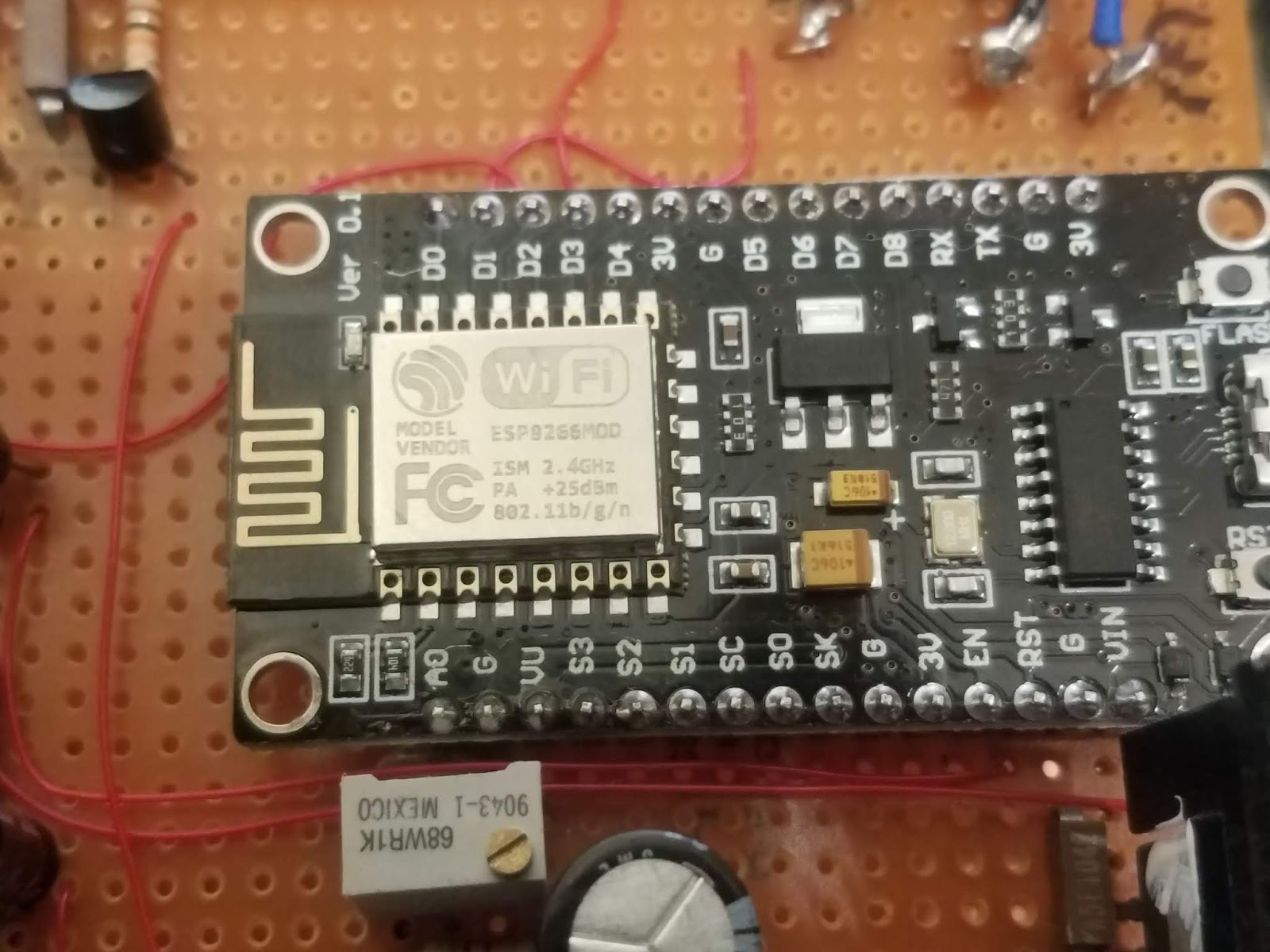
Figure 2:
The "business end" of the small board that contains the
ESP8266 module - the device with the metal shield.
This board also includes a USB plug, a CH340-like
USB to serial converter that allows for programming
and debugging and a voltage regulator that allows direct
operation of this board from a 5 volt supply.
As can be seen here and in Figure 4, the ESP8266 board was,
itself, mounted to a larger prototyping board for construction
of the ancillary circuitry.
Click on the image for a larger version.

On site we do have an Ambient Weather ^(tm) station, but anyone who has used this (or similar) hardware knows that some vendors of this type of gear make it difficult to obtain your own data without jumping through hoops:  Although this data is visually available on the local display or even on a web site, it is a bit awkward to pull this data from their system and (at least with the newer versions of the hardware) one cannot get this data locally from the weather station itself.

Fortunately, the most-needed data - temperature inside the building - is easily measured using inexpensive sensors, so it made sense to throw together a device that could make these measurements and present them in an easy-to-use web interface.

The ESP8266 "Arduino" board:

As is often the case with projects like this, the Internet has the answer.  The ESP8266 is an inexpensive embedded computer module that has a reasonable amount of program memory and RAM and it also sports hardware such as a WiFi module, several digital  I/O pins and a 10 bit A/D converter.  What this means is that for less than U.S.$12 you can get two of these delivered to your doorstep that contain an already-mounted ESP8266 module on a carrier board with a USB port in a format that strongly resembles that of the ubiquitous Arduino development board.  More importantly, the Arduino IDE supports this board meaning that it is pretty easy to use this hardware in your own projects.

Because the '8266 board has been available for quite a while, there is a large library of software for it - including a small web server and code to interface with many types of devices, including the well-known (and relatively inexpensive) DHT-22 temperature and humidity sensor.

Comment:  The ESP8266 variant used here appears to be the "12E" version which has 32 Mbit (4 Mbytes) of Flash memory and "around 50k" of RAM.

The "DHT Humidity and Temperature web server":

It took only a few minutes to find online several implementations of a web server coupled with the DHT-22 sensor - and I chose what seemed to be a popular version on a web site by Rui Santos - to look at it yourself, go here:

randomnerdtutorials.com/esp8266-dht11dht22-temperature-and-humidity-web-server-with-arduino-ide/

Presented in good detail, it was only about 20 minutes from the start to tack a few flying leads to my $6 ESP8266 "Arduino" board to connect the DHT-22 sensor before I had a wireless web server on my workbench that was happily reading the temperature and humidity.

Of course, getting something working can be miles from a finished project and that was certainly the case here as the project was about to be subject to self-inflicted feature creep and code bloat as I'd already decided that I wanted it to do two other things as well:

• Monitor the AC line voltage.  The WebSDR receive site - being rural - suffers from very dirty AC mains power.  We have seen the nominal 120 volt mains exceed 140 volts for brief periods in addition to the frequent outages - and it would be nice to have a device that would allow us to record such excursions.

• Telemeter the gathered information via RF.  Because the ESP8266 is a small computer - and it has data that we want - and we are at a radio receive site - it would be a simple matter to have this unit tap out the information using Morse code on a low-power, unlicensed (part 15) transmitter that was capable of being received by the on-site receivers.

The final result is this, in schematic form:

Figure 3:
The schematic of the support circuitry of the ESP8266 unit described, including a pictorial representation of the processor board itself.
Click on the image for a larger version.

Circuit description:

The ESP8266 is treated as a single component - the support circuit being connected to the pins as noted with the '8266 itself being mounted on a larger board as can be seen in Figure 4, below.  It's worth noting that this is a 3.3 volt device which means that the "high" output voltage is around 3 volts:  If I'd needed a digital input, I would have had to make sure that the logic high input level was appropriately limited in voltage.

Power supply and monitoring:

There are two uneregulated AC-DC transformer "wall warts", both being a low-voltage transformer (9-12 volts AC) with full-wave rectification and capacitive filtering  - one to power the unit and the other to monitor the line voltage.  The separation of these two function is necessary for obvious reasons:  We'd want the unit to continue to function when the AC mains was out, but continue to run from the UPS which means that we can't monitor or own power supply!  Even if we could, the current consumption of the unit varies a bit and as a consequence, so does the unregulated voltage from the monitor supply.  The source of power for the unit itself could be anything that can provide 10-15 volts DC - regulated or not - but these AC->DC transformers were on-hand, plus being simple transformer-rectifier-filter units, they do not generate RF noise - unlike some switching-type devices - a factor important at a radio receive site.

The power from each of the AC-DC adapters enter via a screw terminal strip and immediately passes through a pair of bifilar-wound inductors - the purpose here being to provide RF isolation:  Because this device contains a computer and a low-power transmitter, we don't want any signals on this device from being radiated on the power leads.

The first AC-DC adapter is used to power the unit - a red LED indicating that voltage is present.  Following this is a "bog standard" 5 volt regulator using a 7805 to provide a lower voltage to feed to the "VIN" pin of the ESP8266 board and to run other circuitry on board.

The other wall wart has only a light load - most of the current being consumed by D4, an orange LED used to indicate that the mains voltage being monitored is present.  As you would expect, an unregulated AC-DC supply like this isn't a precision instrument when it comes to measuring line voltage as it is not any sort of RMS measuring device and with its built-in filter capacitor, it's also relatively slow to respond  - but it is "good enough" for the task at hand.

This voltage is divided down via R3 and variable resistor R4 for the 0-3.3 volt input range of the "A0" (analog input) pin on the ESP8266 module.  (Note:  It's reported that A/D range of the "raw" '8266 module is 0-1 volt - apparently this board includes a voltage divider to scale from 3.3 volts.)  Resistor R4 is 10 turn unit used for calibration of the line voltage.

Watchdog timer:

Figure 4:
The completed ESP8266-based temperature, humidity and line voltage
monitoring device.  The CW transmitter portion is in the upper-left corner
of the board with the 555-based watchdog timer below it.  In the lower-
right corner is the 7805 regulator with its heat sink with R4, the
calibration for the line voltage being seen just below the lower-left
corner of the ESP8266 board.  The gray wire at the top connects to the
small board containing the DHT-22 temperature/humidity sensor.
The entire unit is mounted via stand-offs into the lid of the plastic case
depicted in Figure 1.  Inside the lid I placed a sheet of self-adhesive
copper foil that is used as a ground plane to which the input filter
capacitors (C1, C3), the LEDs and the ground connections of the
board are soldered.
Click on the image for a larger version.

Because this device is unattended in a remote location I took the precaution of adding a simple hardware watchdog timer.  The software generates a pulse train (nominally a square wave) on pin "D2" which is then applied to transistor Q1:  Capacitive coupling, via C7, is used as a DC coupled signal would have made it possible that a watchdog reset condition could have been simulated if the pin were stuck "high".  The timer itself is the ubiquitous NE555 "programmed" via C8 and R7/R8 to have an approximately 45 second period.

The pulse train from pin D2 pulses Q1, keeping timing capacitor C8 discharged - but if the pulse train stops, pin 3 will go high after the timing period, briefly pulsing the "RST" (reset) pin of the EP8266 via capacitively-coupled Q2.  A 45 second period was chosen as it takes about 8 seconds for the ESP8266 to "boot up" enough for the software to generate the - and it also allows just enough time to upload the program.

During initial development one would probably not plug a 555 into its IC socket as spurious resets would likely be an annoyance as there may not be code to create the reset pulses, but with the size of the code for this project the reset period is long enough to allow uploading of the code before a reset occurs and the pulses resume.

Temperature/Humidity sensor:

The readily-available DHT-22 sensor is used, chosen over the slightly cheaper DHT-11 as the '22 offers a wider temperature and humidity measurement range - although the software can be configured to work with either one. To avoid erroneous temperature or humidity measurements from the unit's heat generation, this sensor is mounted on its own board as depicted in Figure 3.  On this small board is not only a power supply bypass capacitor (C20) but also a pull-up resistor R19.

The "sensor module" - visible in Figure 1 - was placed inside a small piece of ABS tubing (gray non-metallic electrical conduit) for protection with small pieces of nylon window screen glued to each end to keep out insects, but allow air flow to permit accurate measurements.

CW transmitter:

Because it is a computer - and there was plenty of code space - I decided to add Morse Code generation to provide telemetry that could be picked up by the HF receivers on site.  Stealing my own Morse-generating C code from a 20+ year old PIC project, I made minor modifications to it, using a hardware-derived timer in the main loop to provide a sending clock.  The Morse generating code toggles D3, setting it high to "key" the transmitter.

The signal from pin D3 goes to Q3 which is wired via current-limiting resistor R13 to Q4, a PNP transistor to provide "high side" keying of the unregulated V+ supply.  This voltage is then passed through resistor R14 which provides both a bit of current limiting and, with C12, some R/C filtering to slow the rise/fall of the voltage:  Without it the RF would have been keyed very "hard" causing objectionable "key clicks" on the rise and fall of the RF waveform.  This voltage is used to key both the buffer and the output amplifiers, described below.

The signal source is a 28.57 MHz crystal "can" oscillator module that I found in my junk box.  While I could, in theory, have done CW keying by turning this oscillator on and off, these oscillators aren't designed to be particularly stable and doing so would have caused the oscillator to "chirp" - that is, the short-term frequency drift that occurred when power was applied would have caused an objectionable shift in the received audio tone during keying.

Instead, the oscillator was powered continuously with its output fed to Q5, an emitter-follower buffer:  R15 "decouples" the oscillator from Q5 somewhat and without it, the RF current into the base of Q5 would increase when its collector voltage was switched off causing the oscillator to heat internally, resulting in a frequency shift.  The output of the buffer circuit is then passed via resistive and capacitive coupling to Q6 which is used as the final RF amplifier.  L1 is used to decouple its collector from the power supply while C16 removes the DC voltage from the RF output.  The remaining components - C17-C19 and L2/L3 comprise a low-pass filter resulting in harmonics that are at least 40dB below the fundamental.

This circuit was originally built without Q5, the buffer amplifier, but I had two issues that could only be resolved by its addition:

• Backwave.  Because the oscillator runs continuously, there will inevitably be a bit of leakage - and in CW where it is the very presence and absence of the signal that is used to convey the information, having a rather strong signal when there is supposed to be silence made it difficult to "copy" the code.  When Q6 was turned off, there was enough leakage between its base and collector to offer only about 15 dB of attenuation when the transmitter was "un keyed".

• Oscillator stability.  As noted above, R15 was used on Q5 to limit the current out of the oscillator to prevent frequency drift as buffer transistor Q5 was keyed.  When I'd tried to drive the output (Q6) directly - without a buffer - I had the same problem:  If I coupled enough energy to drive the transistor, the frequency would vary with the CW keying - and the backwave would get worse - but if I increased the resistor enough to reduce the problem, the transistor would be properly driven - which also increased the backwave as the transistor's output would fall in comparison to the signal leakage.

With the circuit built as shown the backwave is at least 40dB below the keyed output  - which is more than adequate for the task.

The code:

As noted above, the basis of the project was that published by Rui Santos - and in the spirit of open source, the code was modified:

• The original code included some small graphics served on the web page - but in line with the KISS principle, this was stripped out in favor of the simplest text, using only standard HTML formatting.

• Additional code was added to read the AC mains voltage via pin "A0".  In the main "loop" routine, this input is read 100 times a second and then averaged, with a new reading made available every second.  This average removes most of the noise on the pin - some of which is internal to the '8266 itself, but the majority of which is due to a small amount of AC ripple on the voltage monitoring line.

• Additional code was added to record the minimum and maximum of all of the monitor parameters - that is, temperature, humidity and line voltage.

• The default of the code was to read the temperature in Celsius, but being in the U.S. I added code to give the readings in Fahrenheit as well. 

• The web server code was modified to display all of the available data - the temperature in Fahrenheit and Celsius, the humidity and line voltage - and their minimum and maximum values.

• Addition modification was made to the web server code to allow each of the data points to be read in simple text format to simplify parsing for remote monitoring and logging of this data.  The nature of the the web server actually made it very easy!

• Yet another modification was made to reset the minimum and maximum readings and to provide information as to how many seconds it had been since a reset had occurred.  The temperature/humidity min/max reset is separate from the line voltage min/max.

• The code also keeps track of mains voltage that falls below a threshold (an outage) or exceeds a threshold (a "surge") - both of which are extremely common at the remote receive site. 

• I added my own Morse generation code, ported from some PIC-based "C" code that I wrote about 25 years ago and interfaced it with the main timing loop.

Source Code:

If you are interested in the source code (sketch) you may find it at THIS LINK.

A few minor changes/improvements - noted in the source code's header - have been made since the original posting.

Implementation:

Figure 5:
 A screen shot of the web page.  This same information is available
from individual links (on the bottom half of the page) that will
return just the information requested, making it trivial to obtain
individual data points using something like WGET.
Click on the image for a larger version.

As mentioned, with the WiFi capability of the ESP8266, the information that this device records is available via a web page on the wireless network:  One only need enter the SSID and wireless password at compile time.  For reasons obvious to anyone familiar with the Internet, this device won't be accessible from the web itself, but only to devices on the local network.

With the CW generator operating on 28.57 MHz, this signal lands within the 10 meter amateur band - and with this device being co-sited with receivers, it is a simple matter of tuning to that frequency to hear the telemetry.  Even though the RF output power is on the order of 50 milliwatts, the actual transmit "antenna" is a very small piece of wire - large enough to radiate just enough signal to be heard via the nearby antennas but not nearly enough to exceed FCC part 15 rules, eliminating the need for this device to transmit an FCC-issued callsign.

Comment:

This device was installed at the Northern Utah WebSDR shortly after this article was originally posted.  You may hear the Morse portion of this device via this link. 

This page stolen from ka7oei.blogspot.com

[END]

A quick look at the QB-300 RF amplifier

Available from many surplus sellers (e.g. via EvilBay) - and (usually) for a reasonable price - is the QB-300 RF amplifier.  Originally made by Q-Bit corporation, this same device has borne several different manufacturers markings over the 30+ years since it was introduced - but it is (pretty) much the same device.

Figure 1:
The BNC-connectorized version of the QB-300.
This appears to be the "original" version, actually made by Q-bit
Corporation.  The voltage specification is slightly ambiguous, being
shown as "+15/24 Vdc".
Click on the image for a larger version.

Having several of these on-hand I decided to take a quick look at its apparent performance - with the general specifications for this device being listed below for your convenience:

• Frequency range:  1 MHz-300 MHz
• Gain:  23dB (or 24.5 +/- 1 dB, depending on source)
• Gain flatness:  1 dB
• Noise figure:  3.8dB (frequency not specified)
• Input/Output VSWR:  <=1.5:1
• Power output (1dB compression):  +22dBm
• 3rd order Intercept:  +37dBm
• Current consumption:  155mA (voltage not specified)

Depending on which data sheet you consult, there are a few discrepancies - for example:

• The data sheet from "API Technologies" shows the input/output return loss as 1 dB - clearly a typo.

• The maximum voltage rating is all over the map:  Some versions of the data sheet show a maximum of 20 volts, others show 24 volts.  The units that I have clearly show the voltage rating as being "+15/24Vdc" and the equipment from which it was pulled provided 24.0 volts.

Knowing the provenance of this equipment, I would have no problem running my amplifier from 24 volts, but based on the ambiguity of the data sheets, I would operate a version that did not explicitly specify 24 volts ONLY from 15 to 18 volts.

A quick test:

Curious about a few aspects of these amplifiers I decided to test it with my DG8SAQ Vector network Analyzer, checking its gain versus frequency in the input matching (e.g. S11) - the results being displayed in Figure 2, below:

Figure 2:
A sweep of the amplifier from 100 kHz to 500 MHz showing the apparent gain and input matching over the frequency range.  Because the DG8SAQ and the interconnecting cables are increasingly imperfect with increasing frequency, expect increasing uncertainty in the S11 readings above 100 MHz or so.
The gain, S11 and VSWR values at specific frequencies can be seen in the upper-left corner.
Click on the image for a larger version.

Of particular interest was the usability of this amplifier above and below its "official" frequency range - and we can see that it's probably useful down to at least 250 kHz and above 450 MHz, albeit at reduced performance (e.g. lower gain, maximum output power, increased noise figure, increased input VSWR.)  Specifically, I measured, below the 1 MHz minimum frequency specification:

• The gain at 285 kHz was still above 21dB - a bit more than a 2 dB drop from the peak gain.  The input VSWR was still below 1.5:1.
• The gain at about 200 kHz was around 18.7dB
• The gain at about 173 kHz was around 16.8 dB and the VSWR had increased to about 2.7:1. 

Above the 300 MHz maximum frequency specification:

• The gain was above 22dB at 400 MHz
• The gain was about 21 dB at 440 MHz
• The gain was around 18dB at 500 MHz.

The reader is reminded that it is likely that above and below the rated frequencies that the maximum output power - not to mention noise figure - is likely to degrade.

Gain versus operating voltage:

Figure 2 was captured with the unit operating at 18 volts and readings were taken at lower voltages, comparing the gain - but your mileage may vary:

• Gain dropped by approximately 0.1 dB at 15.0 volts.
• The gain was about 0.2 dB lower at 12.0 volts than at 18 volts.
• The gain was about 1 dB lower at 8.0 volts than at 18 volts.
• The gain was about 5 dB lower at 5.0 volts than at 18 volts.
• The amplifier began to exhibit signs of low-frequency instability below 5 volts.

Although not directly measured, one should expect the maximum output power (P1dB) and the intercept point to drop below the specifications when operating it from lower than 15 volts:  The amplifier is likely to be perfectly usable in the 12-14 volt range, but it's likely marginal at 8 volts and below.

A peek under the hood:

Popping the top cover, we see this:

Figure 3:
A look inside the QB-300 amplifier:  The input and output is on the left and right sides, respectively.
Click on the image for a larger version.

 It is immediately apparent that this is not a run-of-the-mill consumer device:  Rather than a circuit board, the unit is built onto an alumina substrate with both soldering of components and spot welding of wires being used.  Two RF transistors are obvious:  The black, 3-lead device near the upper-left corner and the white ceramic device marked with "Q-21" just to its right.  The rest of the components are likely related to feedback/equalization as well as regulation of the operating and bias voltages for the RF devices.

Clearly, it's not hermetically sealed or conformally coated, so  weather protection is certainly warranted if this were to be operated outside.

Uses for this amplifier:

This amplifier was designed as a general-purpose gain block in the HF-VHF range, but it is likely useful into the low UHF range meaning that it should work from the 630 meter amateur band (on the low end) into the 222 MHz - and possibly the 70cm - amateur bands on the high end.

For general HF (amateur radio) amplification purposes, it should be an excellent performer - provided that one keeps in mind that it's gain may be a bit too high in certain applications in that a signal input level of a around -5dBm will push it into overload - and off-air signals of this strength might appear from:

• Local AM broadcast stations.  Especially on a long wire antenna (longwire, rhombic, end-fed half-wave) these signals can, by themselves, overload the amplifier if you live anywhere near  a transmitter.  A simple high-pass filter can effectively reduce such signals and prevent overload.

• High-power shortwave stations.  On a good antenna, signals on the 49, 41 and 31 meter band can be extremely strong in Europe and some parts of the U.S.

If you have strong signals that could overload the amplifier, beware using an attenuator on the input of the amplifier in your receive system.  As an example, if you wish to be able to hear the background noise at 10 meters to be able to hear the weakest possible signals you will need to make sure that your system noise figure is no more than about 15dB - but if you had a cable loss of 3 dB in "front" of your amplifier (between the antenna and the amplifier) and you used a 10dB attenuator in this signal path, you are already at 13dB - and the nominal 3.8 dB of noise figure of this amplifier will push that number to about 16.8dB meaning that your system noise will now likely be high enough that you can no longer hear atmospheric noise if you are fortunate enough to be in a very "RF quiet" location.

In short:  If you hear more noise when you connect your antenna system to your receiver system than when you connect it to a dummy load, you are OK - but if you can't hear the difference, your system will not be sensitive enough to hear the weakest signals.

For receive-only purposes it is often the case that with a low-noise amplifier, a good, quiet (in terms of noise) receive antenna will not need to have much gain from the antenna itself - and if the gain is low, you are less likely to intercept enough absolute signal power to overload the amplifier.  Here are just two of the many possible examples of antennas to consider:

• Small receive loop.  This type of antenna - usually around 3 feet (1 meter) diameter for MF and HF use can offer local noise rejection as well as the ability to null signals from directions broadside the plane of the loop.  This type of antenna will have negative gain (e.g. less than 0 dBi) but its performance can be quite good with a decent, low-noise amplifier like the QB-300.  For an antenna like this, one would place the amplifier at the antenna to minimize cable losses.

• Beverage on the ground.  Also known as the "BOG" antenna, this is simply a wire - as long as possible - laying on the dirt and working against a good (and electrically quiet) ground consisting of one or more ground rods and counterpoise wires and its feedline electrically decoupled (with a "current" balun) to prevent noise from the shack from being brought to the antenna.  This antenna - mostly useful in rural areas - is reported to work well overall despite the likely "negative" gain.  As with the receive loop, it's best to place the amplifier at the antenna feedpoint.

Amplifier and receiver protection:

It should go without saying that any amplifier (or receiver) connected to a large antenna should be preceded by adequate lightning protection to prevent damage to the amplifier from wind static/discharge and nearby lightning strikes as depicted in Figure 4, below.  Such filtering should be placed after any filtering that might precede the amplifier.

Decent protection can be had with four ordinary silicon diodes - two series pair connected anti-parallel (back-to-back) with a bleed resistor (4.7-100k) to shunt voltages above about 1.2 volts.  It's worth noting that the amplifier itself would already have overloaded before signals can a high enough level to cause the diode protection to conduct and cause distortion!

Figure 4:
Depiction of simple input protection circuitry.
On the left, the diodes ("D") are ordinary silicon diodes connected in series for approximately 1.2 volts of conduction.
On the right, a common full-wave rectifier module is used with its DC "output" shorted, providing an equivalent to the circuit on the left.  It is suggested that a low current (2-5 amp) rectifier be used.
The voltage rating of the diodes is not particularly important - a 50-100 volt rating being just fine.
Resistor "R" is not critical and can be anything from 4.7k to 100k and it is used to dissipate any accumulated DC in case the antenna itself does not have a DC ground.  An inductor can be used in addition to or instead of "R" - a value of 22-100uH (e.g. 8-10 turns on an FT50-75 toroid) being suitable for 630-10 meters.
Click on the image for a larger version.

Provided that one avoid excessive signal input level, it can also be used as the basis for a receive multi-coupler.  For example, following the amplifier with an 8-way RF splitter - which, itself, will have a loss of around 10dB - the overall gain will be in the range of 14dB while preserving the system's overall noise figure to allow reception of weak signals on the higher HF bands.

This page stolen from ka7oei.blogspot.com

[End]

A "curiously sharp" 40 meter band-pass filter to reduce 41 meter SWBC overload.

At the Northern Utah WebSDR (sdrutah.org) we recently added another server (WebSDR #4) that is connected to an existing east-pointing beam antenna on site. This antenna, it is hoped, will better-allow users to hear stations on the 40-10 meter bands in the eastern U.S. and, to a lesser extent, the DX locations to which it is pointed.

Figure 1:
East-pointing beam antenna at the Northern Utah WebSDR.
This antenna has 10-13 dBi gain and signals in the 39,41
and 31 shortwave broadcast bands can be extremely strong!
Click on the image for a larger version.

As one would expect, this antenna has gain - between 10 and 13 dBi, depending on the frequency - and this has implications when propagation between Utah and the Eastern U.S. is favorable:  Already-strong shortwave broadcast (SWBC) signals become even stronger.

Because the S-meter (signal meter) on the receivers have known calibration it is possible to make an indirect measurement of some of these signals' strength and, at times, individual signals have been observed in the -20 to -15 dBm range at the antenna - these levels being in the "60 over S-9" range.  At times - particularly during evening "gray line" propagation (where both the transmit and receive sites are entering/in twilight/evening) signals can peak significantly.  What's worse is that there may be several such signals, increasing the total RF power impinging on the receiver risking not only receiver overload, but also providing a ready source of multiple, modulated carriers to mix together and reappear within the receiver's passband among the desired signals.

These sorts of signals are far above those that might be expected due to amateur-only transmissions owing to the widely disparate signal levels.  For example, a very well-equipped "DX" stations may be able to run 1500 watts of RF into a (monster!) 15 dBi gain antenna and attain an EIRP (Effective Isotropic Radiated Power) in the area of 50kW, but this does not compare with an SWBC station which may be running 500kW peak (about 125kW carrier) into an antenna with (a conservative) 18dBi gain - an EIRP of about about 32 million watts - a signal level nearly 1000-fold (30dB) stronger than one that would be transmitted by law-abiding amateurs.

What's worse is that some of these SWBC bands are adjacent amateur bands - and the 40 meter amateur - which runs from 7.0-7.3 MHz is no exception as the 41 meter SWBC band is just above it, starting at 7.3 MHz.  With such close spacing, typical filtering in receivers have little hope in effectively rejecting these nearby, strong signals.

Addressing the problem:

There are two time-honored ways of dealing with strong signals impinging on receivers:

• AGC (Automatic Gain Control):  This circuit "monitors" the signal level at the receiver and automatically reduces the gain when they exceed a certain amount.  In the past, this has been applied only to signals within the passband of the receiver's IF to keep the audio level constant regardless of the actual signal strength, but this is also applied to modern SDRs where the level of the entire passband of signals being input to the A/D converter is monitored and adjusted to prevent overload. 

• RF front-end filtering:  With the advent of solid-state radios starting in the 60s and 70s the design of RF filtering used in amateur receivers began to be wideband, typically covering MHz, rather than a narrow peak.  This was done not only because it was easier to do so with these designs, but also because it allowed "general coverage" reception outside the amateur bands and it was significantly less expensive than mechanically-complicated, ganged tuning systems - but it had the down-side that signals some distance away frequency-wise could still cause the receiver to experience overload.  These days - particularly with modern, high-performance direct-sampling Software-Defined Radios (SDRs) - "narrow" filtering is once again being used, along with AGC, owing to the need - more than ever - to strictly control the total amount of RF energy reaching the A/D converter to prevent overload. The receiver used at the Northern Utah WebSDR is a type of SDR where the RF energy is converted directly to audio and then digitized.  This has the advantage of simplicity, but it lacks the "AGC" circuit meaning that it is possible for strong, off-frequency signals to cause overload of not only the RF circuits, but also the audio circuits and the A/D converter.

While it is possible to add an AGC circuit to this receiver system to prevent overload (this has been done with some of the other receivers on site - and is still an option) the first step that we are taking is to build a "sharper" filter.

The "Curiously Sharp" band-pass filter:

Passing signals on the 40 meter amateur band - which ends at 7.3 MHz in the Americas - and filtering out signals on the 41 meter shortwave broadcast band - which starts at 7.3 MHz - is a tricky proposition:  How does one suddenly go from passage of signals to blocking them within just a few 10s of kHz?

Figure 2:
The completed 40 meter band-pass filter
in a Hammond 1590D die-cast box.
Click on the image for the larger version.

The answer is:  You don't - but you do the best that you can!

The limiting factor in constructing a "brick wall" filter - one that has an abrupt transition - is physics and is intrinsic to real-world components:  Real-world inductors have ohmic resistance and capacitors have dielectric losses - to name but two factors - that limit the unloaded "Q" of the circuits.

What does this mean?  A truly "sharp" filter will ultimately be limited in its performance by these factors:  One must trade off insertion loss and/or filter performance in terms of how quickly our band-pass filter cuts off.

Fortunately, the first of these - insertion loss - is pretty easy to mitigate:  Have enough extra signal gain in the receive system to accommodate the insertion loss.  At 40 meters, we have "signal to burn" - partly because our receive antenna has so much gain, but there is also a "strong" (resistant to overload) RF amplifier located near the antenna to mitigate the effects of cable losses at the higher HF bands (10 meters).

Even if we didn't have both antenna and amplifier gain, we could afford to lose a lot of signal at 40 meters:  A system noise figure of about 30 dB (assuming a unity gain antenna) is sufficient to "hear" the noise on even a quiet band, so a significant loss can still be made up by placing an RF amplifier after the filter and still be able to resolve the 40 meter noise floor during quiet band conditions.

Figure 3:
 Schematic of the 40 meter bandpass filter.  This is a 7-element Elliptical (Cauer) filter centered at 7.15 MHz - the middle of the U.S. 40 meter amateur band.  It was originally designed with the aid of the "A.A.D.E. Filter Design" program, version 4.5 being available from the AE5X web site.
The nominal impedance of the filter portion is 800 ohms to permit higher values of inductance and lower values of capacitance in an effort to ease construction and to reduce component losses (e.g. reduce the L/C ratio).
Click on the image for a larger version.

Figure 3 shows the schematic of the filter - and a few explanations are warranted.

• ALL of the capacitors must be either NP0 (a.k.a. C0G) ceramic or silver mica capacitors - preferably the latter.  I did not use any silver mica capacitors, but I used known-good ceramic capacitors from a trusted source (e.g. Mouser-Key) rather than from a random EvilBay seller.
• L1, L4 and L7 were wound using solid 12 AWG copper wire.  The wire that I used happened to be tin-plated, but enameled copper wire will be just fine with only the two ends (and the tap point) being bared for soldering.  If bare copper wire is used it is suggested that it be very clean and sprayed with clear lacquer after construction is completed to prevent oxidation.
• The other inductors were wound using 17 AWG wire, which was on hand, but 18 AWG would be fine.
• All of the inductor/capacitor pairs have their own resonant frequency, noted on the diagram in parentheses.  The 7.15 MHz resonances (C1/L1, C4/L4, C7/L7) will be adjusted very close to the stated frequency but the other resonances (C2/L2, C3/L3, C5/L5, C6/L6) are made adjustable by small ceramic (or air) variable capacitors and must be CAREFULLY adjusted for the proper filter response.
• As can be seen, the filter's in/out ports are terminated with 2dB resistive attenuators to help assure a consistent source/termination impedance to the filter and prevent the likely-imperfect devices to which it is connected from too-badly affecting the response.
• L1 and L7 show taps that are chosen to be at the 50 ohm points.  The "S11" port of a known-calibrated VNA may be used to best-set the 50 ohm points of the taps during filter construction/adjustment.

Constructing the filter:

Figure 5, below, shows the as-built filter:

During construction I used my DG6SAQ Vector Network Analyzer - and a tool such as this is invaluable as it will give "live", dynamic readings to facilitate adjustments.  The more economical (approx. $50 U.S.) "NanoVNA" will work fine (along with the "NanoVNA Saver" program) - and although its update/sweep rate is quite a bit slower than that of the DG6SAQ, it's still usable.  No matter what sort of VNA you might use, be aware that the limited number of data points per scan can "hide" details such as narrow, deep notches - and this is especially true with the NanoVNA.

The "through loss" measurements (in dB) were the most important in this case as the insertion loss versus frequency plots over a range of about 6.5 to 7.8 MHz allowed the "dialing in" of the resonant circuits.  During construction two "bloody ended" coaxial cables were used - one end of each being connected to the VNA and the other end having its ground shield tacked to the ground plane and the center conductor attached to the point under test:  These test cables are visible in Figure 4, below.  This "plywood and foil" test bed allowed an easily reconfigurable circuit design and test bed for ideas - and, most importantly, it helped me determine if a particular design was even practical.

Figure 4:
Early prototype built on a piece of plywood covered with self-adhesive
copper foil.  Originally, L1, L4 and L7 were wound on toroids - but
a switch was made to the larger, air-wound inductors to reduce losses.
This early version used input/output transformers for transformation of
the 50 ohm in/out to the 800 ohm (nominal) impedance of the filter itself -
but this was changed to tapped inductors as that was simpler and
lower loss.  This simple "breadboard" allowed several ideas to be tried
before settling on the final version, giving plenty of room to work.
This picture shows the short pieces of coaxial cable that were
tacked to the foil ground:  These cables connect to the two
ports of the VNA used to analyze the response of the filter.
 Click on the image for a larger version.

The first to be constructed were the large resonators (L1/C1, L4/C4, L7/C7) which needed to be set to 7.15 MHz and for this, two resistors (1k-4.7k - the precise values are unimportant) were connected in series with the center point connected at the "top" end of the parallel L/C network and the "ends" being connected to the VNA's in and out ports.  With this arrangement one can see the "peak" where the L/C circuit resonates - the two resistors minimizing loading - and one compresses/stretches the large inductor using a small screwdriver to increase spacing between turns or a pair of needle-nose to compress them - or, if necessary, removes fractional turns - to "dial it in" at 7.15 MHz.

After these have been adjusted, the other L/C networks are then constructed - and this is where it gets to a bit tricky:  The variable capacitors allow the resulting "notch" to be moved around, but it may be necessary to add/remove turns from the inductor - or add small amounts of capacitance (10pF at a time) to get the circuit's adjustment within range of the variable capacitor.  In some cases, one may temporarily "shunt" (short out) one or more of the series L/C networks to better-visualize the notch that one is trying to adjust.  If you can't find the "notch", don't forget that it may be above/below the sweep range and you may temporarily need to set the start/stop frequencies wired to find it.

As often happens, one's first ideas don't work quite as expected:  You will note that in Figure 4, L1, L4 and L7 are shown as being toroidal inductors, but it became clear that these inductors were just too lossy, a factor that severely affected "Q" and performance.  I ended up using air-core inductors wound from much heavier wire as can be seen in Figure 5 to minimize loss.  Ideally, superconducting inductors would have been used, but for some reason such devices that operate at room temperature aren't available!

Adjusting such a filter requires patience as everything interacts.  An examination of Figure 5 will reveal that each section is connected with jumper wires, allowing isolation of the individual tuned circuits.  Eventually, one can get a "feel" for how the adjustments interact - but it may still be necessary to  disconnect the sections and check/tune them individually back to a starting point if one gets "lost" and the response/tuning gets worse and worse.

Also visible in Figure 5 are shields around the large tuning elements made from pieces of double-sided copper-clad PC board material.  While shielding between the sections isn't really necessary from a performance standpoint, placing the filter - which was constructed on the lid of the Hammond 1590D box - into the box itself causes the filter to detune slightly due to proximity to the enclosure's walls:  The shielding on the sides of the large coils - and the bars across the top - "simulated" the filter being within the die-cast box and almost eliminated the effect, but still allowed access to permit adjustment if the large coils.

Figure 5:
As-built 40 meter band-pass filter.
This filter was constructed on a solid copper ground plane of circuit-board material.  to hold components in place and to isolate junctions from the ground.  "Manhattan" (island) pads were used for junctions that needed to be isolated from the ground:  The "Me Pads" (from "QRPMe") were used.  Blobs of RTV are used to mechanically support some of the larger components.
Click on the image for a larger version.

 

To be clear:  This should NOT be your first band-pass filter as it is VERY tricky to adjust - and you MUST have available a scalar and/or vector network analyzer to properly adjust it!  If both of these do not apply to you it is suggested that you obtain help - or prepare to get this gear and pull your hair out during adjustment!

Did it work?

The answer is Yes.

Figure 6:
A sample passband of the filter during adjustment:  The ultimate adjustment resulted in a somewhat flatter response.
The "upper" notches (L2/C2 and L5/C5) can clearly be seen as can the upper "lower" notch (L6/C6).
The intrinsic insertion loss, including the two 2 dB pads, is around 15dB.  The ultimate rejection is around 65 dB, correlating to a filter rejection of around 50 dB, taking into account the through losses.
Click on the image for a larger version.

 

This filter offers over 20dB of (additional) attenuation below 6.9 MHz and above 7.4 MHz and between careful adjustment of the receive system gain (e.g. just enough signal to comfortably "hear" the noise floor during the quietest part of the day) and the attenuation of the 41 meter signals, overload on the 40 meter receivers on the Northern Utah WebSDR #4 no longer occurs.  If you wish, you can check it yourself, particularly during the evening "gray line" hours when sunset is sweeping across North America at sdrutah.org.

Comments:

The use of a similar filter in ITU Regions 1 and 3:

In Regions 1 and 3 the 40 meter amateur band covers 7.0-7.2 MHz with strong SWBC signals starting at 7.2 MHz.  Narrowing this filter to 200 kHz would require a redesign and would further-push the limits of standard components, but broadly similar results should be possible.  Alternatively, the center frequency of this filter design could be moved down by 100 kHz to 7.05 MHz and offer similar rejection to signals above 7.2 MHz.

Options for even "sharper" filtering:

While the filter described is starting to push the limits in terms of the use of reasonably-obtainable components, there is another option:  A frequency-converting band-pass filter.  For this, a local oscillator and a pair of mixers would be used to convert the 7.0-7.3 MHz 40 meter passband down to a lower frequency where a "sharper" filter would be easier to construct.

For example, using an 8 MHz oscillator would convert the 40 meter band from 7.0-7.3 MHz to 0.7-1.0 MHz, inverting the frequency, meaning that the most critical part of our filtering - that "above" 7.3 MHz - would now be happening below 700 kHz.  Of course, this "converting filter" would have to have decent band-pass filtering of its own to prevent response to undesired signals and the mixer used for the down-conversion would have to be adequately "strong" to withstand the insanely strong 41 meter signals.

Once the filtering is done at this lower frequency, the same 8 MHz oscillator would be used to up-convert back to 40 meters:  With the same oscillator used in both directions, it need not be particularly frequency-stable as any drift would be self-compensated.

This page stolen from ka7oei.blogspot.com

[End]

About the WSPRDaemon noise graphs - and repurposing for use in monitoring WWV(B) signal levels over time.

What is WSPRDaemon?

The WSPRDaemon program is largely a work of Rob, AI6VN and it exists for the purpose of facilitating the reception of WSPR signals off air, processing the data, and making that data available publicly - not only to wsprnet.org, but also via the wsprdaemon.org web site.  The WSPRDaemon script runs on a Linux computer - typically a Raspberry Pi - and typically takes data from a web-connected receiver (typically a KiwiSDR) - but it can also use the ubquitous RTL-SDR dongle or even the "raw" audio input from a receiver via a sound card.

For each of the (approximately) 2 minute receive "cycles" of WSPR transmissions (which are, worldwide, scheduled to start precisely at the beginning of each even-numbered minute) an audio (.wav) file is recorded for each receiver - and this audio is then processed using the "WSJT-X" program to decode the WSPR transmissions found within that audio stream.

Features not found in WSJT-X that are made available in the wsprdaemon script include the scheduling of receivers (e.g. switching a limited number receivers to most favorable bands) and the "merging" of several receivers - possibly using different antennas for diversity - that are listening to the same band so that only the best of the WSPR "spots" is reported, avoiding duplicate reports of a given transmission.

• More information about wsprdaemon may be found on the wsprdaemon Github page.
• For more about WSPR, see the WSPR Wikipedia page and the other pages to which it links - especially K1JT's page.

What it does:

While not precisely calibrated, having long-term, disparate records of WSPR signal reception from all over the world can provide useful information to amateur radio operators and researchers alike, providing a glimpse into the propagation of LF, HF and even VHF (and higher bands) which can help divine when propagation is occurring between two stations and when it occurred.  Having a "live" and past database of these events can help validate/tweak models of the Earth's geomagnetic field and its interaction with the sun on the ionosphere - and to satisfy the intellectual curiosity of anyone who wishes to study this by themselves.

Accumulation of "noise" data:

In addition to the accumulation of WSPR data, the wsprdaemon software is able to measure the apparent noise floor on the specific frequencies associated with WSPR transmissions on the amateur bands and with some hardware it is possible to calibrate this measurement in absolute terms of intercepted noise power.

If receivers taking these readings are found at disparate "RF quiet" sites around the world, this data can be informative of the natural, background noise which can be indicative of the state of the ionosphere and the Earth/Space environment:  In some cases, it is possible to observe the rising/setting of strong radio noise sources such as Sagittarius A and, occasionally, "noisy" planets in our solar system such as Jupiter not to mention the tremendous noise that can result when the Earth's magnetic field is being abused by our local star.

The software makes two separate noise measurements:

• The noise "floor" within the passband.  This reading (the "RMS" level, in Red on the wsprdaemon.org graphs) is the calculated noise floor level and its processing attempts to "remove" the effects of other signals within the detection passband.

• The signal power within the passband.  This reading (the "FFT" level, in Blue on the wsprdaemon.org graphs) is the total power within the passband.  Unlike the RMS reading, this is indicative of the cumulative power intercepted and will always be higher.

Even though the apparent detection bandwidth of these receivers is on the order of 400 Hz, all readings are scaled (by approximately 26 dB) such that the power readings reported are relative to a 1 Hertz detection bandwidth.

A typical graph may be seen below:

Figure 1:
A typical graph showing the last 24 hours of noise on the 40 meter amateur band a receiver at the Northern Utah WebSDR.

The displayed time, in UTC, shows the noise level rising at around local nighttime and then dropping off at night.  This graph is "skewed" somewhat by the overnight presence of strong thunderstorms in the Eastern United States, the intensity of which gradually tapered off overnight and into the day and by the fact that the antenna used is a log periodic beam has significant gain that is pointed in the direction of those storms.

Almost the "inverse" of this is the noise graph from another receiver at the Northern Utah WebSDR site:

Figure 2:
This graph depicts a 24 hour plot of the noise floor on the 20 meter band.

The noise floor can be seen to increase during the daylight hours, but drop to the floor during the night when propagation and ionospheric stimulation by the sun effectively ceased.  As expected - particularly during the period of low sun activity during which this is being written - the noise floor and signals decrease during local nighttime.

In theory, careful analysis of the noise data used to produce the above graphs can provide the opportunity to analyze HF propagation modes and the effects of Earth-Space environment.

Monitoring signals from consistent sources:

It occurred to me that the wsprdaemon script also afforded the opportunity for something else for which it was originally intended - the monitoring of consistent signal sources of known transmitter power and location.  From the Utah location, one source of signals - those from the NIST in the form of the WWV and WWVB  transmitters - was obvious.

A quick modification of the wsprdaemon script allowed the addition of additional frequencies:  While there would clearly be no WSPRnet reporting on these non-amateur channels, the noise measurements would still be posted as the graph below depicts:

Figure 3:
 A noise graph of the WWVB transmission at 60 kHz in Fort Collins, Colorado.

The red line shows the received signal level from WWVB - the same signal used to set many automatic clocks - on 60 kHz.  During daylight hours the signal level is pretty consistent at the "-100dBm" mark while during the night, signal levels vary a bit - particularly during sunrise/sunset where ionospheric perturbations are evident.

The "Blue" line is largely influenced by the 17dB amplitude modulation of the WWVB carrier used to convey time and date information, but it is also prone to being "diluted" by peaks in the background noise as can be seen during the nighttime hours (from about 0400-1100 UTC) where propagated lightning static is evident.

From the same site, on a frequency that is orders of magnitudes higher we get this plot:

Figure 4:
 A noise graph of the signal and noise levels on the 10 MHz WWV/H frequency.

The graph of Figure 4 is a bit more cluttered as one might expect.  The Red "line" shows the wildly varying signal of the signal on 10 MHz - which could be from either WWV in Colorado OR WWVH in Hawaii.  As is the nature of HF, these signals can vary significantly - not only between day and night, but also from one moment to the next.  The blue line generally depicts the noise level at 10 MHz, but this may not be truly representative as it may be being affected by the ever-present modulation on the WWV/H carrier - primarily in the form of the 100 Hz time code modulation.

The utility of the graph in Figure 4 may be debatable as there is not one, single signal source, but it does provide a general perception of the signal levels that one might expect - and how the time of day affects them.

Final comments:

In addition to the general monitoring of the noise floor on the HF bands where WSPR monitoring is taking place, the wpsrdaemon script can also be used to monitor signals from known transmitters.  To be sure, this wasn't the intended use of this software and if such data is useful, it's likely that the utility and accuracy of such measurements could be improved.

* * * * * * * * * * * * * * * * *

Modifications to the wsprdeamon script for version 2.8a:

In the "wsprdaemon.sh" file, one need only add a few lines to the code to produce the "new" bands in the array "WSPR_BAND_LIST", as in:

"WWVB        58.5"
"WWV_2_5  2498.5"
"WWV_5      4998.5"
"WWV_10     9998.5"
"WWV_15    14998.5"
"WWV_20    19998.5"
"WWV_25    24998.5"
"CHU_3       3328.5"
"CHU_7       7848.5"
"CHU_14     14658.5"

Each new "band" is named by the first entry on the line (e.g. "WWVB") and the frequency of the carrier that one wishes to monitor is defined in kHz in the second entry.  Note that the frequency used here is 1.5 kHz lower than the actual carrier frequency to be monitored.

In the "wsprdeamon.conf" file where the receiver and its use is to be defined, these "bands" - defined in wsprdaemon.sh - are used in exactly the same way as any other band in the list.  For example, one might schedule the start a hypothetical receiver called "KIWI_1" on the WWVB signal at 0000 local time as follows:

declare WSPR_SCHEDULE=(
"00:00  KIWI_1,WWVB"
)

Comment:  At present, wsprdaemon will dutifully try to process the audio file for WSPR spots - but it will fail to do so.  It should be possible to modify the code to add an argument that will prevent this from happening to reduce processor loading.

* * * * * * * * * * * * * * * * *

This page stolen from ka7oei.blogspot.com

[END]